Radiation Geometry

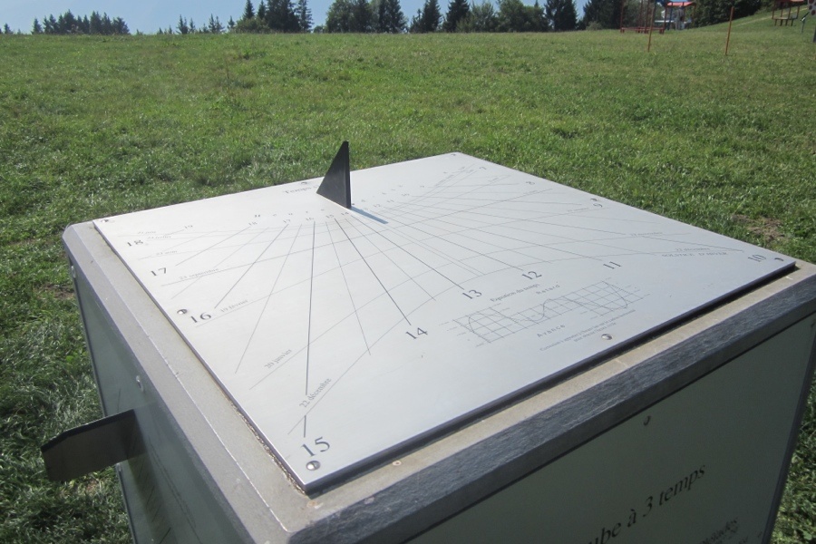
The position of the Sun in the sky and the path of the solar beam.

Radiation Geometry

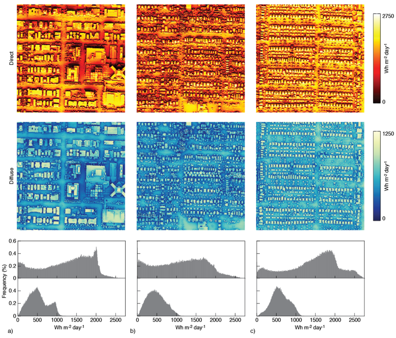
Processes of absorption, reflection and scattering of radiation through the atmosphere determine the available short-wave radiation reaching Earth’s surface.

Photo: A. Christen

Address survey concerns

Learning Objectives

• Be able to predict the relative position of the solar disk.
• Use this to calculate the irradiance reaching our planet ‘at the top of the atmosphere’ (in absence of atmospheric effects).

Earth’s Climate System: Energy Inputs

Table 1: Average heat flux density from external sources at Earth’s surface

Surface	Average Energy Flux
Solar electromagnetic radiation	241.5 W m-2
Energetic particles (sun and space)	0.001 W m-2
Geothermal	0.06 W m-2
Anthropogenic (fossil fuels, nuclear energy)	0.02 W m-2

What drives our climate system and provides energy for all life on Earth.

Motivation

• The geographic distribution of radiant energy is not equally distributed on Earth:
  • Large scales (Earth’s geometry)
  • Small scales (topography)
• Those differences cause many microclimates.

Photo: A. Christen

Wh = one watt (1 W) of power expended for one hour (1 h) of time strong energetic gradients.

Radiation applications

Radiation Properties and Laws

• Dual properties: wave/particle.
• Frequency ν, wavelength λ and speed of light c.
• The electromagnetic spectrum
• Reading package Lecture 4-5 ‘Radiation Basics’

Electromagnetic waves. Radiation can be described as a form of energy due to the rapid oscillations of electromagnetic fields. The oscillations may be considered as travelling waves characterized by their wavelength λ (distance between successive wavecrests). Radiation is able to travel in a vacuum, and all radiation moves at the speed of light (c=3×108 ms−1), and in a straight path. Hence, instead of wavelength, we can express radiation by its frequency ν (in oscillations per second, i.e. s−1) (v = c/λ) We’re typically concerned with 0.1 to 100 μm with visible from 0.4 to 0.7 μm Particle properties. Radiation can be also described by discrete bundles of energy that have properties similar to particles. Quantum physics tells us that radiation is transferred as discrete packets called quanta (or photons if in the visible part of the spectrum). Energy of quantum is e = h ν. (h = Plancks constant (6.63 × 10-34 J s)) Plants can only use photons in the visible range of the spectrum which is also called photosynthetically active radiation (PAR, 0.4 - 0.7 μm).

Radiation Properties and Laws

• Energy of a photon¹

• Plank’s law²

• Stefan Boltzmann law³

• Wien’s Law⁴

• Kirchhoff’s Law⁵

\[ e = hv \qquad(1)\]

\[ E = \frac{2*h*c}{\lambda^{5}}*\frac{1}{e^{\frac{h*c}{\lambda*\sigma_b*T}}-1} \qquad(2)\]

\[ E_b = \sigma_b T^4 \qquad(3)\]

where \(\sigma = 5.67 * 10^-8\)

\[ \lambda_{max} = \frac{b}{T} \qquad(4)\]

\[ \zeta_{\lambda} = \epsilon_{\lambda} \qquad(5)\]

Shortwave vs. Longwave

All bodies possessing energy (i.e. whose temperatures are above absolute zero, 0 K = −273.2◦C) emit radiation. Total radiant heat energy emitted from a surface is proportional to the fourth power of its absolute temperature Wein’s displacement law: It states that a rise in the temperature of a body not only increases the total radiant output, but also increases the proportion of shorter wavelengths of which it is composed. Kirchhoff’s law: Emissivity = absorptivity

Sun-Earth Geometry

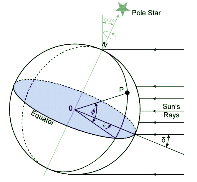
Solar declination (\(\delta\)): Angle between Sun’s rays and equatorial plane.

Latitude (\(\Phi\)): Angle between the equatorial plane and the site of interest (point P in the figure).

Hour angle (h): Angle through which the Earth must turn to bring the meridian of the site P directly under the Sun. It is a function of the time of day.

Declination: The earth’s equator is tilted 23.45 degrees with respect to the plane of the earth’s orbit around the sun, so at various times during the year, as the earth orbits the sun, declination varies from 23.45 degrees north to 23.45 degrees south. This gives rise to the seasons. Meridian: meridian (or line of longitude)

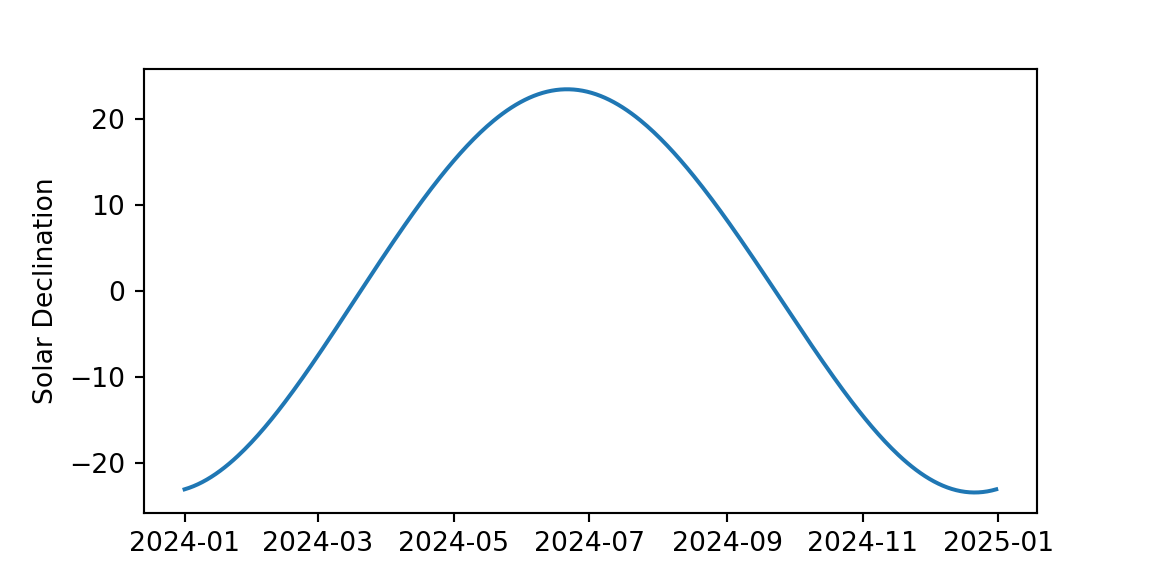
Calculating Solar Declination

\(\delta\) only depends upon day of year, which gives returns \(\delta\) in radians

• The equation is complex due to the non-circular orbit of Earth

\[ \begin{eqnarray} \delta = & 0.006918 - 0.399912 \cos( \gamma)+0.070257 \sin( \gamma) \\ & -0.006758 \cos(2 \gamma) + 0.000907\sin(2\gamma) \nonumber \\ & -0.002697\cos(3\gamma)+0.00148 \sin(3\gamma) \nonumber \end{eqnarray} \qquad(6)\]

where \(\gamma\) is the fractional year and DOY is the day of the year:

\[ \gamma = \frac{2 \pi }{365} (DOY-1) \qquad(7)\]

One radian is just under 57.3 degrees. Radians = 180/pi The declination angle, denoted by δ, varies seasonally due to the tilt of the Earth on its axis of rotation and the rotation of the Earth around the sun

NOTE: Simple approximation has angle in radians (2pi) whereas answers to study questions has it in degrees (360).

Calculating Solar Declination

import numpy as np
import pandas as pd
import matplotlib.pyplot as plt

def Solar_Declination(DOY):
  gamma = 2*np.pi/365*(DOY-1)
  delta = 0.006918 - 0.399912 * np.cos(gamma)+0.070257 *np.sin(gamma)-0.006758 *np.cos(2*gamma) + 0.000907*np.sin(2*gamma)-0.002697*np.cos(3*gamma)+0.00148 *np.sin(3*gamma)
  return(delta*180/np.pi)

Dates = pd.date_range('2024-01-01','2024-12-31')
Declination = Solar_Declination(Dates.dayofyear)
plt.figure(figsize=(6,3))
plt.plot(Dates,Declination)
plt.ylabel('Solar Declination')

Radians = 180/pi -The declination angle, denoted by δ, varies seasonally due to the tilt of the Earth on its axis of rotation and the rotation of the Earth around the sun. -declination is zero at the equinoxes (March 22 and September 22), positive during the northern hemisphere summer and negative during the northern hemisphere winter. 

iClicker

What is the solar declination on June 21st?

• A 23.45 \(^{\circ}\)
• B 0 \(^{\circ}\)
• C -13.45 \(^{\circ}\)
• D 18.45 \(^{\circ}\)
• E -23.45 \(^{\circ}\)

Observer’s local geometry

Solar Zenith (Z) Angle between Sun’s rays and observer’s local zenith.

Azimuth angle (\(\Omega\)) Angle between projections onto local horizontal for both Sun rays and true North (0=360°).

Solar Altitude (\(\beta\)) Angle between Sun’s rays and observer’s local horizon (\(\beta\) = 90°- Z)

Calculating the Zenith

\[ \cos(Z) = \sin(\beta) = \sin(\Phi)\sin(\delta)+\cos(\Phi)\cos(\delta)\cos(h) \qquad(8)\]

where the hour angle (h) is a function of local apparent time (LAT):

\[ h = 15^{\circ}(12-LAT) \qquad(9)\]

Beta = altitude angle Angle through which the Earth must turn to bring the meridian of the site P directly under the Sun. It is a function of the time of day. 360/24

So many times…

• Coordinated Universal Time (UTC): standard time, referenced to mean solar time at the prime meridian.
• Standard Time (LST) - What is on your watch without daylight savings offset - same for all longitudes within a given time zone.
• Local Mean Solar Time (LMST) - Mean solar time is fixed and ensures that on average, highest solar altitude is observed at noon (not at each day of the year). Changes with longitude.
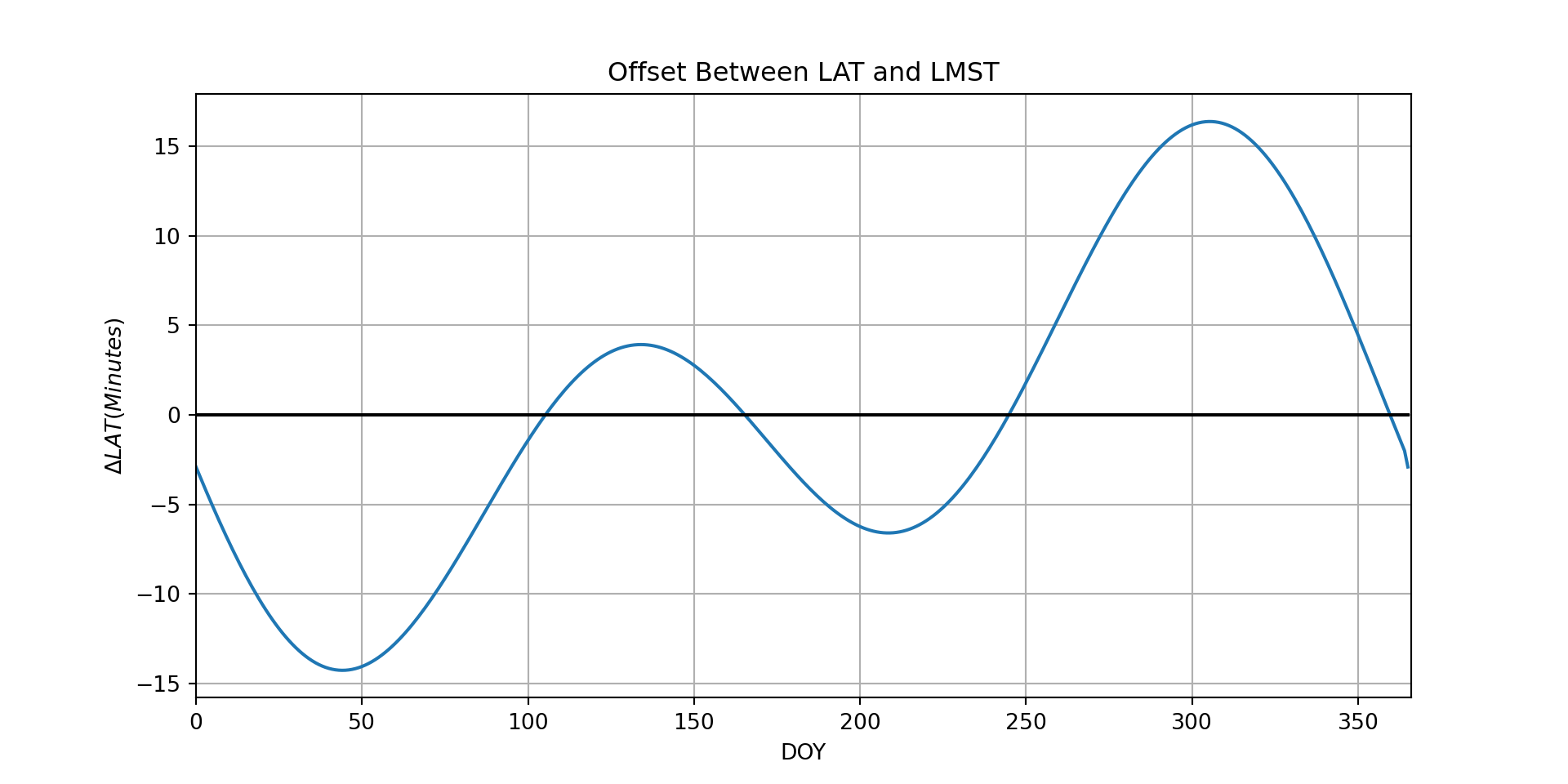
• Local Apparent Time (LAT) - A non-uniform time that varies through the year according to the equation of time. It ensures that highest solar altitude is always observed at noon.

Local Mean Solar Time

Add (subtract) 4 min to LST for each degree of longitude east (west) of the standard meridian of the time zone.

• On the central meridian of -120 \(^{\circ}\) PST = LMST
• Any other longitude within time zone has an offset of 4 min per 1º between LMST and PST

So Many Times

\[ LMST = (TZ) + (\lambda-TZ_{m})\frac{4}{60} \qquad(10)\]

where \(\lambda\) is longitude, \(TZ\) is time in LST (e.g., PST = UTC-8) in hours, and \(TZ_{m}\) is the central meridian for a given time zone (e.g., PST = -120 \(^{\circ}\)). You can then calculate the local apparent time LAT as:

\[ LAT = LMST-\Delta LAT \qquad(11)\]

and \(\Delta LAT\) is: \[ \begin{eqnarray} \Delta LAT = & 229.18[0.000075+0.001868\cos(\gamma)-0.032077\sin(\gamma) \\ & -0.014615\cos(2\gamma)-0.040849\sin(2\gamma)] \end{eqnarray} \qquad(12)\]

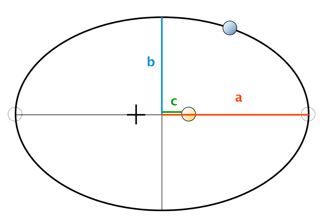
Planetary Orbits and Kepler’s Laws

Kepler’s first law: states that planets follow an elliptical orbit, with the Sun in one focus. This implies that the Earth-Sun distance is changing during a year.

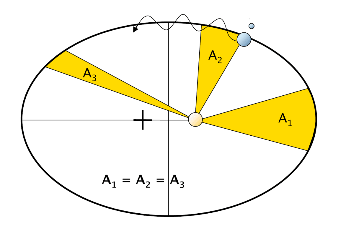
Kepler’s second law: a planet moves fastest when it is near the perihelion and slowest when it is near Aphelion.

Perihelion (January) = closest to sun Aphelion (June)

Local Apparent Time

Timezone not provided, estimating for -127.5, 50

(0.0, 366.0)

Local Apparent Time

Photo: A. Christen

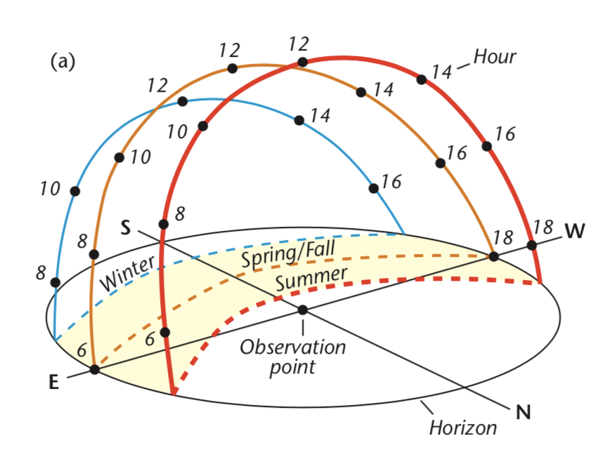
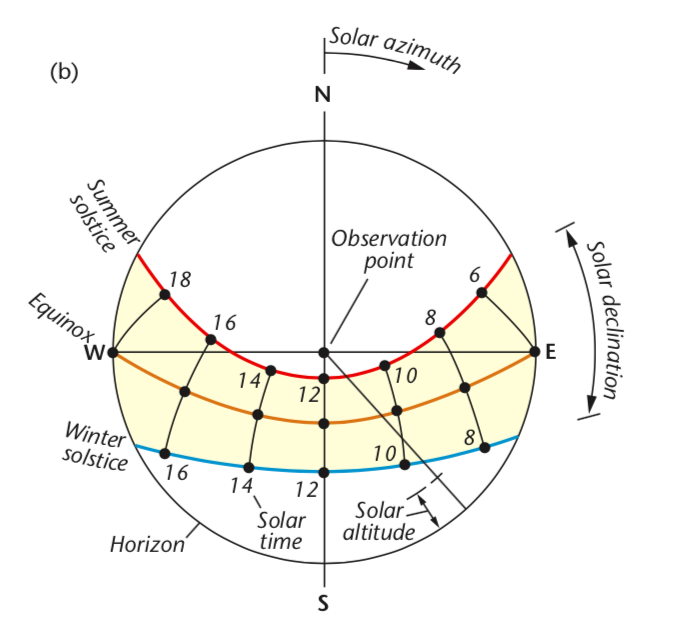
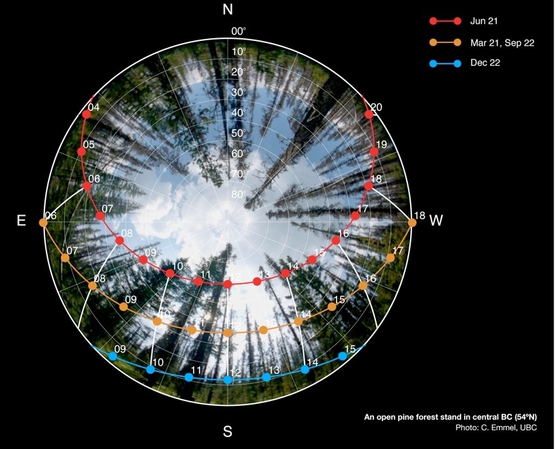
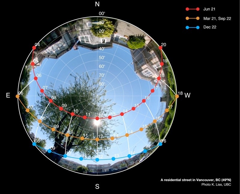
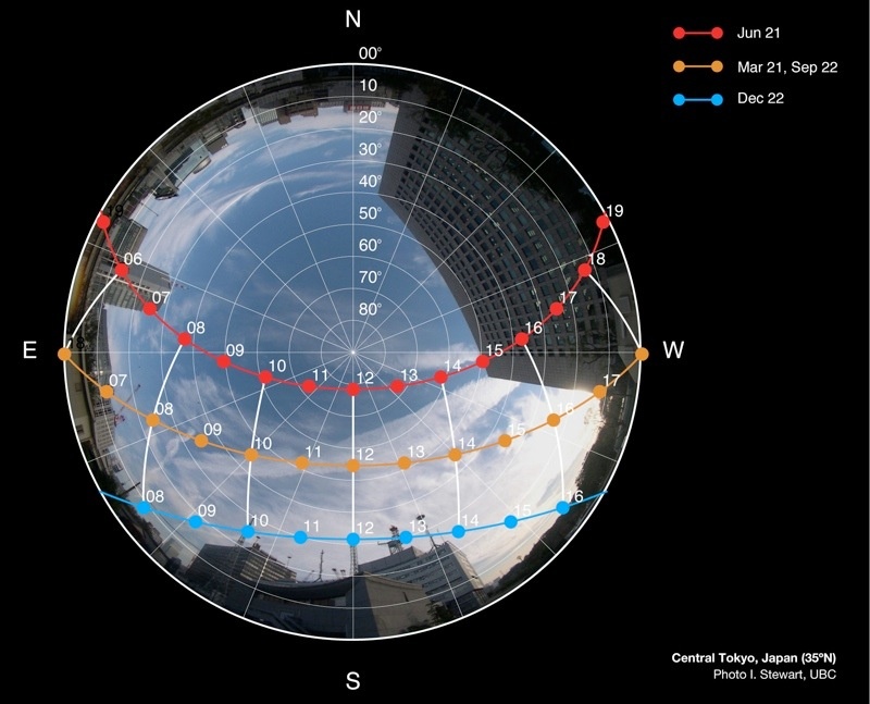
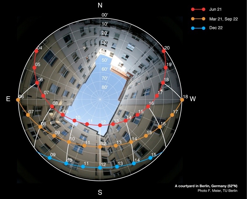
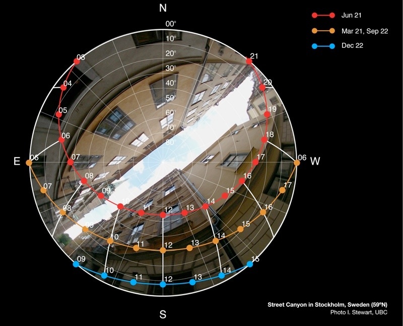
Sun path diagrams

Paths of the Sun across the sky vault for a mid- latitude location in the Northern Hemisphere at the times of the solstices and equinoxes

The projection of (a) onto a two- dimensional plane thereby forming the basis of a Sun path diagram.

Altitude = 1-solar zenith angle (Angle between Sun’s rays and observer’s local horizon) Solar azimuth angle = Angle between projections onto local horizontal for both Sun rays and true North (0=360°).

Solar altitude angle

http://ibis.geog.ubc.ca/courses/geob300/applets/sunpath/index.html https://www.esrl.noaa.gov/gmd/grad/solcalc/

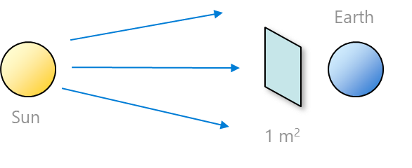
Cosine Law of illumination

\(R_p\) the radiative flux density on a surface perpendicular to the beam and Z is the zenith angle of incidence (i.e the angle between the surface and the direction of the beam).

\[ R_s = R_p cos(Z) \qquad(13)\]

Solar constant \(I_0\)

The radiant flux density (irradiance) at the top of the atmosphere normal to the solar beam an at Earth’s mean distance from Sun.

• Present observations suggest \(I_0 \approx 1361 W m{-2}\)

The Nimbus satellite hosted the first instruments measuring the solar constant(NASA).

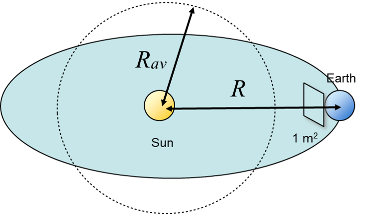
Earth’s Distance to Sun

\(R_av\) is the mean distance Earth-Sun over the year and \(R\) is the actual distance Earth-Sun at a given time.

-Area ratio -Energy spreading over area -gamma = 2pi/365(DOY-1)

Extraterrestrial Irradiance

The solar input at top of the atmosphere at any time and location hence is given as \(I_ex\): \[ I_{ex}=I_0(\frac{R_{av}}{R})^2\cos(Z) \qquad(14)\]

where \(I_0 \approx 1361 W m^{-2}\), \(\cos(Z)\) applies the cosine law of illumination, and \((\frac{R_{av}}{R})\) adjusts the solar constant Earth’s elliptic orbit:
\[ \begin{eqnarray} (\frac{R_{av}}{R})^2 = & 1.00011+0.034221\cos(\gamma)+0.001280\sin(\gamma)+\\ &0.000819\cos(2\gamma)+0.000077\sin(2\gamma) \end{eqnarray} \qquad(15)\]

Take home points

• We discussed a lengthy recipe to predict the relative position of the sun with reasonable accuracy, taking geometry and astronomical parameters into account.
• We combined cosine law of illumination (GEOB 200, ATSC 201) with the solar constant to calculate extraterrestrial irradiance at any given time and for any location.
• In the next lecture we will add the effects of the atmosphere with the goal to predict surface irradiance.