Assignment 4
GEOS 300, 2024
See the Answer Key Here
There is no template for this assignment, you can use a .ipynb or .Rmd file from one of your previous assignments as a template to get started.
Instructions
It is strongly recommended that you complete the assignment in Python or R, although you can complete it in excel/numbers if necessary. They will download the data for you and get you started with a few blocks of code to make plots and tables. If you are electing to complete the lab in excel, you can find all the relevant data files here here. Note these data are in .csv format. If you plan to work in excel, you should save a copy of the data in a suitable excel format (e.g., .xlsx) before making any charts or doing any calculations.
Please upload your answers including all calculations, discussions, tables, and graphs in a single document (PDF or HTML file). Note that you can download your .ipynb file under ‘File \(\gg\) Download as \(\gg\) HTLM or PDF via Latex’ and submit this as your report. Label the report document with your name and your student number. Upload your answers to Canvas. Do not attach a spreadsheet.
Make Sure your student number is include on each plot you produce, and that each plot is using the correct units.
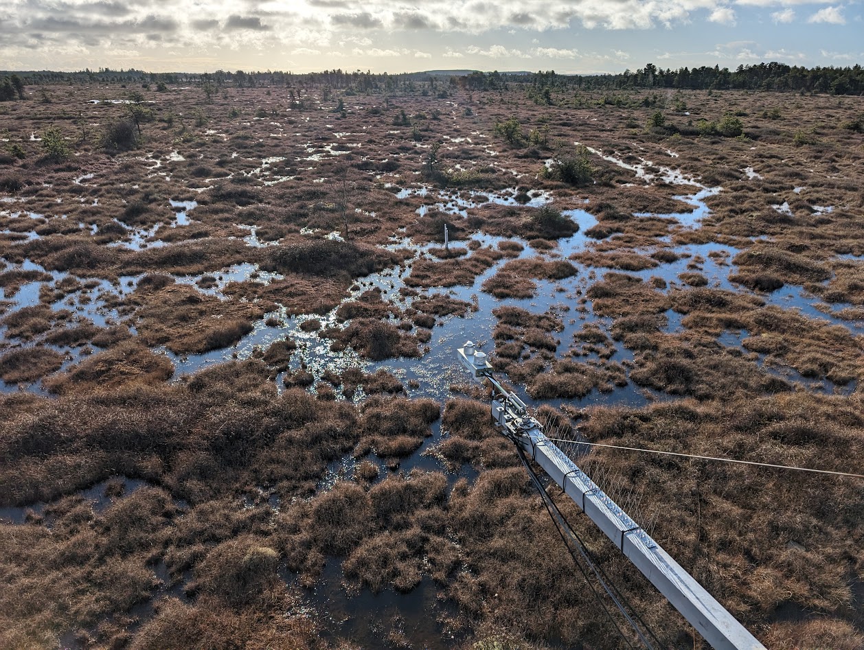
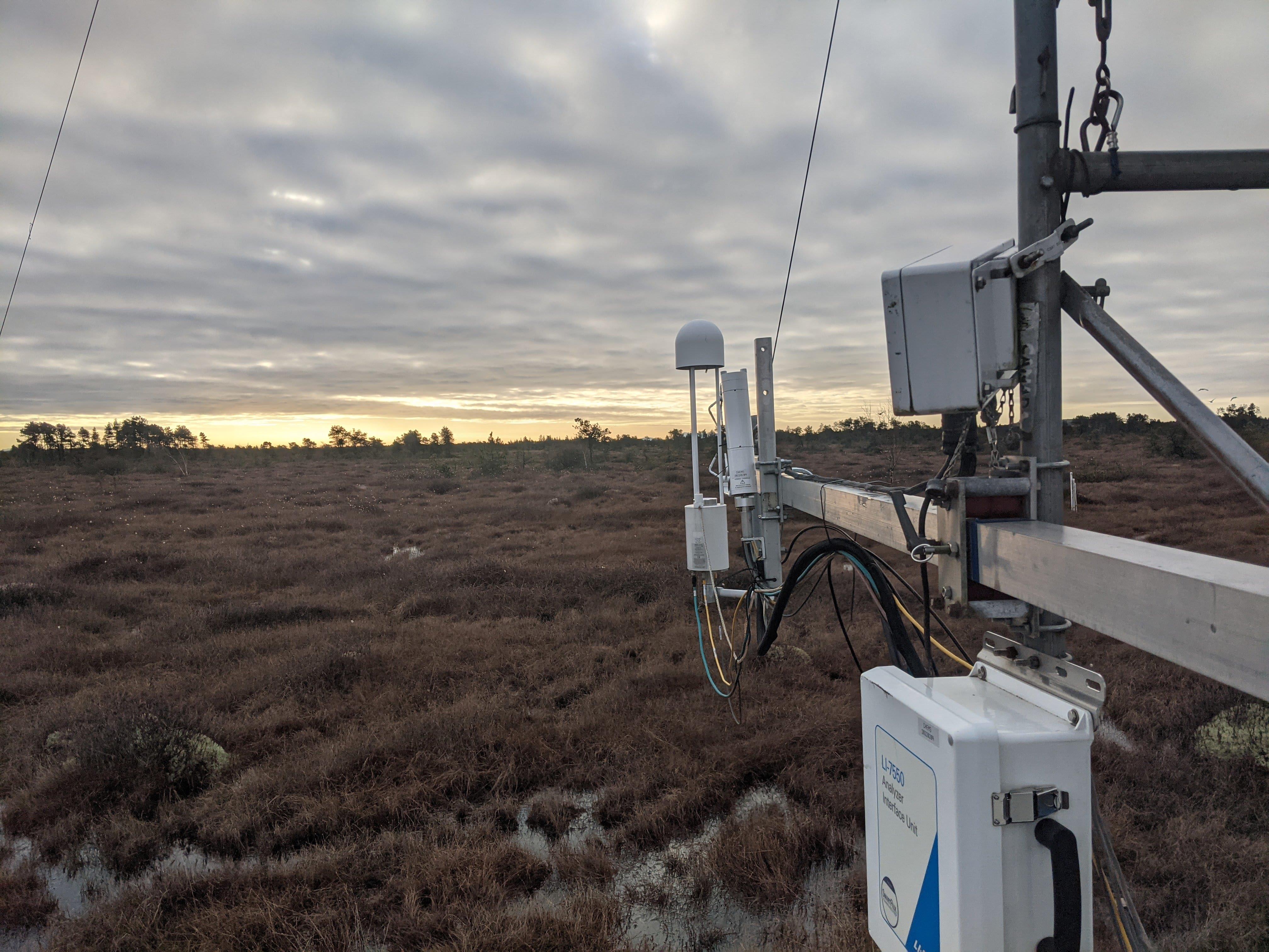
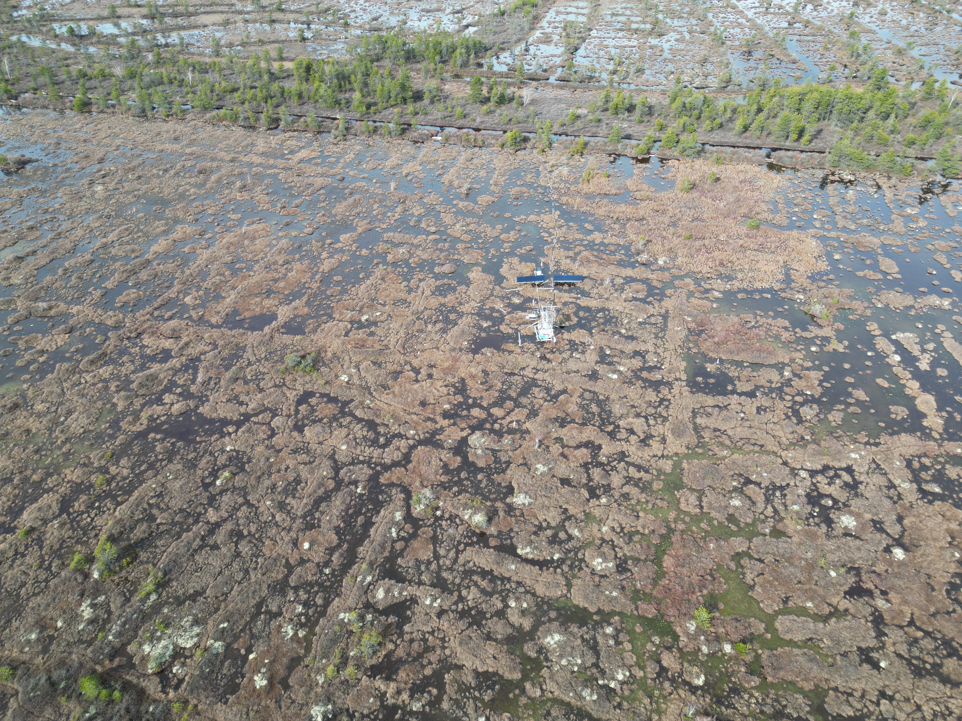
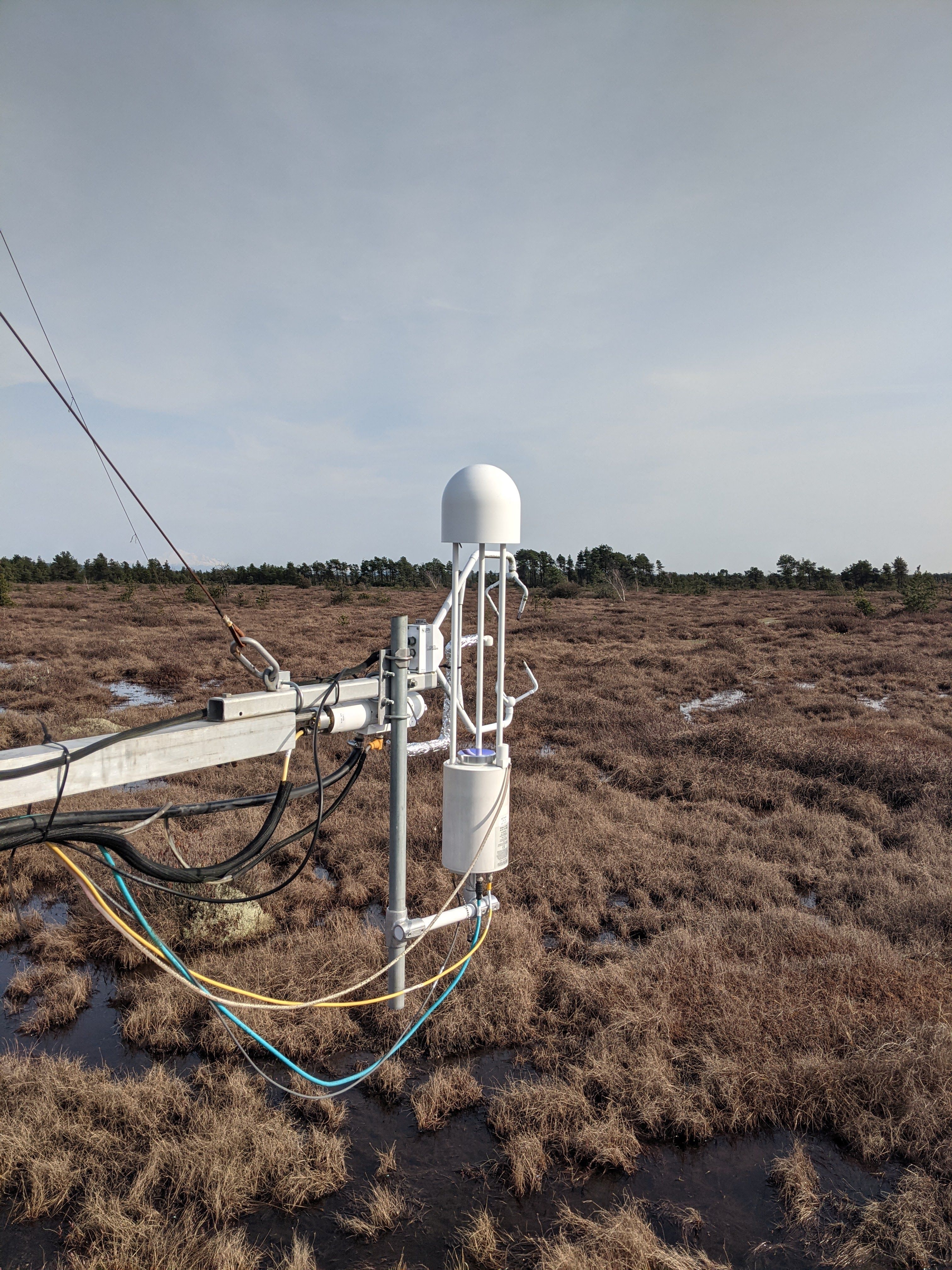
CA DBB Flux Station
In this lab, assignment, you’re going to go back to look at more data from the CA-DBB (aka “BB”) Eddy Covariance (EC) Station located in Delta, BC. We’re going to look specifically at a single day of EC observations to consider how the energy and mass flow through the ecosystem over a daily cycle.
Figure 1 shows some pictures of the site from different perspectives. Figure 2 shows an interactive web map with high resolution satellite imagery. Clicking on “BB” in will zoom to the CA-DBB station and show the site’s “Flux Footprint Climatology”, which is the average “field of view” of the eddy covariance system at the station. Clicking the “BB” button again will toggle the footprint later on and off. You can pan/zoom to get a feel for what the site looks like. Take note of the scale bar in the bottom left to get a sense for how large the footprint is. Table 2 shows the estimated size of the source area contours.
| Source Area % | Size \(m^2\) |
|---|---|
| 90% | 13845 |
| 75% | 2569 |
| 50% | 587 |
The data-set includes half-hourly values of the following variables: absolute temperature \(\overline{T}\) at 0.4 m and 2 m above ground in \(^{\circC}\), mean horizontal wind \(\overline{u}\) at 0.4 and 2 m above ground in \(m s^-1\), net all wave radiation \(R_n\) at 5 m above ground in \(W m^{-2}\), air pressure \(P_a\) in \(kPa\), photon flux density in \(\rm{\mu mol}\,\rm{m}^{-2} \rm{s}^{-1}\) and measured covariances \(\overline{u^{\prime}w^{\prime}}\), \(\overline{w^{\prime}T^{\prime}}\), \(\overline{w^{\prime}\rho_v^{\prime}}\), and \(\overline{u^{\prime}\rho_{\rm{CO}_2}^{\prime}}\), all measured at 2 m above ground using an eddy covariance system. Here \(u^{\prime}\) and \(w^{\prime}\) are instantaneous horizontal and vertical winds in \(m s^-1\), respectively, \(\rho_v\) is absolute humidity in \(\rm{g}\,\rm{m}^{-3}\), and \(\rho_{\rm{CO}_2}\) is the molar density of the greenhouse gas carbon dioxide (in \(\rm{\mu mol}\,\rm{m}^{-3}\)).
| Last digit of student number | filename |
|---|---|
| 0 | 20160620.txt |
| 1 | 20160808.txt |
| 2 | 20160811.txt |
| 3 | 20160812.txt |
| 4 | 20160813.txt |
| 5 | 20160817.txt |
| 6 | 20160729.txt |
| 7 | 20160730.txt |
| 8 | 20160820.txt |
| 9 | 20160821.txt |
Question 1
Download your data and print descriptive statistics for all columns. How do maximum and minimum air temperature at 0.4 m compare to those at 2.0 m?
Question 2
Convert the air temperature \(T\) values at 0.4 m and 2.0 m to potential temperature \(\theta\). Recalculate the descriptive statistics for \(\theta_{z=0.4}\) and \(\theta_{z=2}\); how does this adjustment impact the values?
Question 3
From the data-set provided, calculate \(H\), \(LE\) and \(F_{CO2}\) from the covariances of \(\overline{w^{\prime}T^{\prime}}\), \(\overline{w^{\prime}\rho_v^{\prime}}\), and \(\overline{w^{\prime}\rho_{\rm{CO}_2}^{\prime}}\) respectively. You can assume that the specific of air is 1.01 kJ kg-1 K-1. You can estimate the density of air \(\rho\) using the Ideal Gas Law Equation 1 and you can estimate the latent heat of vaporization following Equation 2:
\[ PV=nRT \tag{1}\]
here,\(R\) is the ideal gas constant (\(8.31446261815324 Pa\ m^3\ mol^{-1} K ^{-1}\)), \(T\) is temperature (in Kelvin!), \(P\) is air pressure, \(V\) is volume, \(n\) is the amount of the gas in mols; with \(n=m/M\), where \(m\) is mass and \(M\) is the molar mass. The molar mass of air is \(\approx .028964 kg mol^{-1}\)
Following Yao & Rogers (1996), the latent heat of vaporization of water (\(L_v\) in \(J g^{-1}\)) can be approximated as a function of temperature (\(T\) in \(^{\circ}C\)) using a third order polynomial function:
\[ L_v = 2500.8-2.36T-0.0016T^2-0.00006T^3 \tag{2}\]
Question 4
Create a graph with time of day on the \(x\)-axis and the three measured flux densities of the surface energy balance (\(R_n\), \(H\), \(H\)) on the \(y\)-axis. Briefly discuss their diurnal course. Do \(H\) and \(LE\) sum to \(R_n\)? If not, why?
Question 5
For 16:00, Calculate \(H\) based on the aerodynamic method using the simultaneously measured profiles of \(\overline{u}\) and \(\overline{T}\). How does the value of \(H\) compare to \(H\) calculated from \(\overline{w^{\prime}T^{\prime}}\)? Why could it differ?
Question 6
Using the covariances and the profile measurements, calculate the eddy diffusivities for sensible heat \(K_H\) and momentum \(K_M\) at 16:00. Is Reynold’s analogy fulfilled or not at 16:00?
Question 7
For 16:00, calculate the Obukhov-length \(L\) and the stability parameter \(\zeta = z/L\). Is \(\zeta = z/L\) really indicating `neutral’ as assumed in using the aerodynamic method above?
Question 8
In the process of photosynthesis, energy is extracted from photons in the PAR range. To assimilate one mole of \(\rm{CO}_2\), it requires an energy of 469 kJ. The same amount is released back during respiration (metabolism, decomposition of organic matter). We call this energy flux density the net biochemical energy storage \(\Delta P\). Calculate \(\Delta P\) at 13:00 in \(\rm{W}\,\rm{m}^{-2}\). At 13:00, what fraction of \(R_n\) is used up in the process of photosynthesis? Is \(\Delta P\) a relevant term in the surface energy balance of this bog or not?
Question 9
Determine the average carbon dioxide (\(\rm{CO}_2\)) flux density between the bog and the atmosphere for this day and convert it to \(\rm{g}\,\rm{CO}_2\,\rm{m^{-2}}\,\rm{day}^{-1}\). Is the surface a net sink or net source for atmospheric \(\rm{CO}_2\) on this day? Note: the molar mass of \(\rm{CO}_2\) 44.01 \(g mol^{-1}\)
Extra Credit: Self guided field trip
Note the extra credit is due with the final exam. Don’t submit the extra credit with Assignment 4! There will be a space to upload your extra credit on canvas in the exam! The total value of the extra credit is yet to be determined, it will depend on how many people complete it and how much thought goes into the responses.
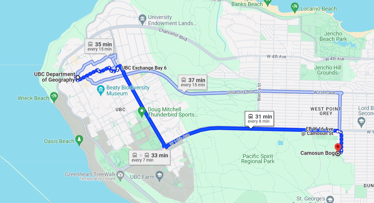
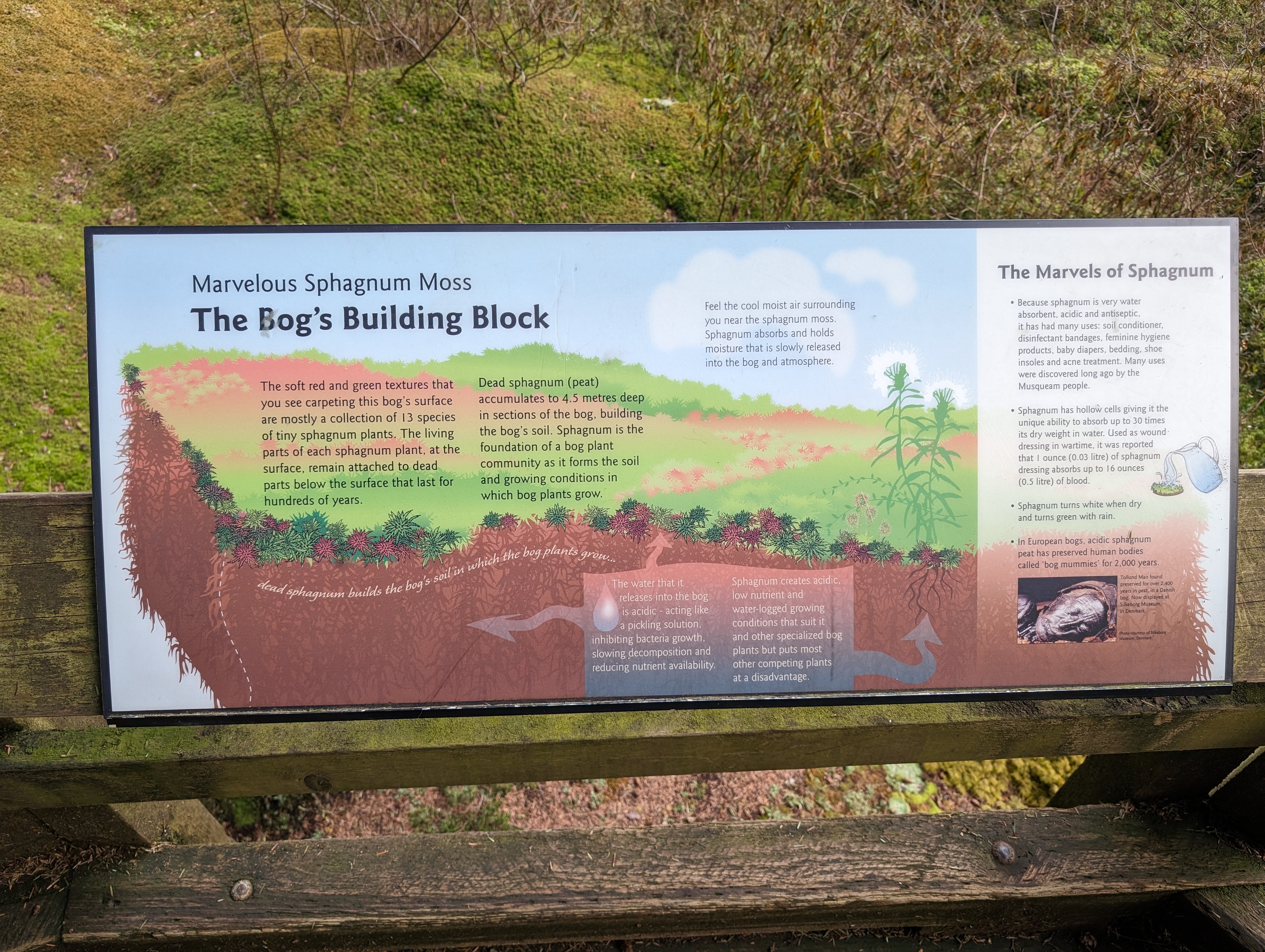
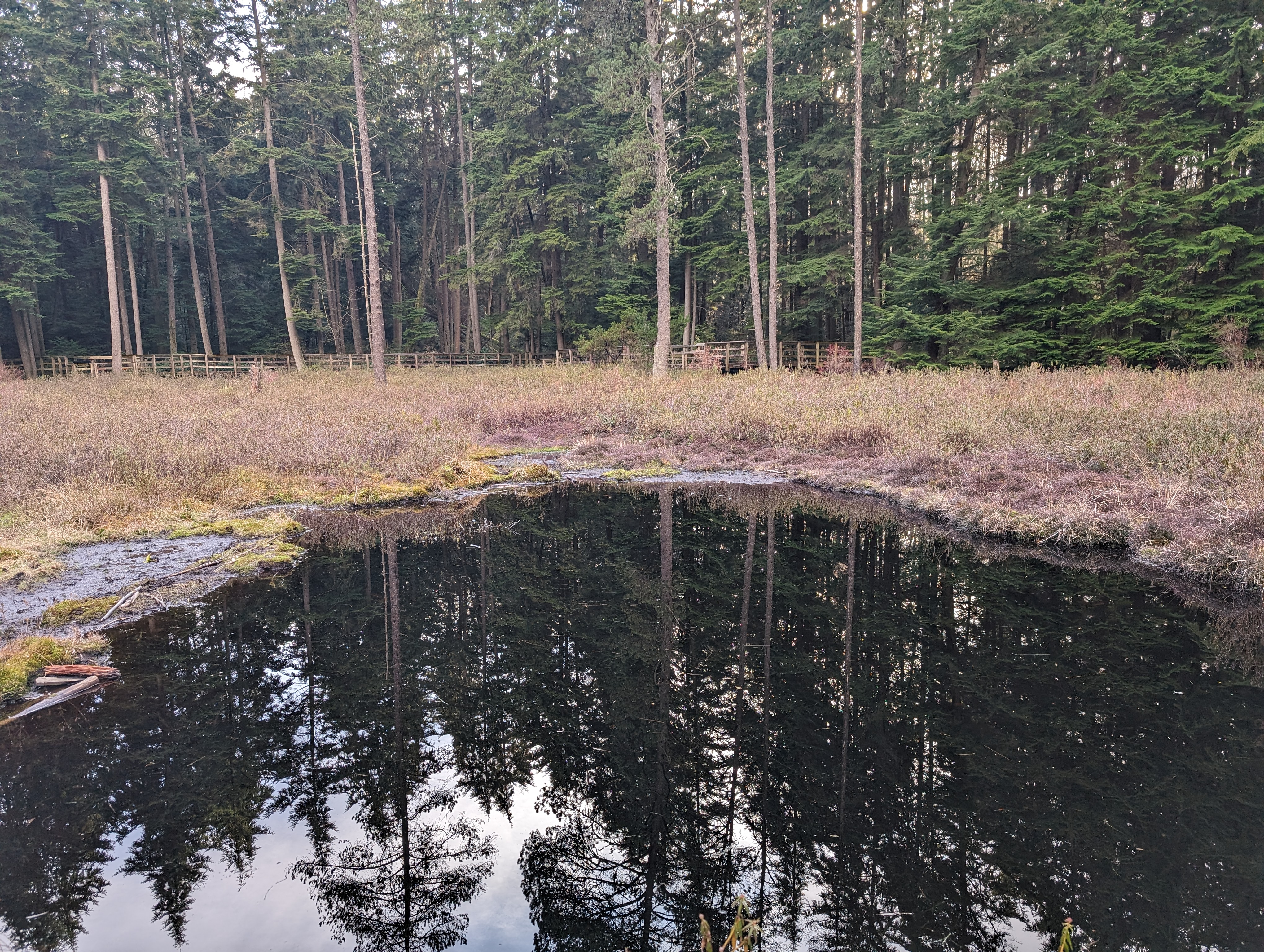
The CA-DBB eddy covariance station is located within the Burns Bog Ecological Conservancy Area. It is a large peatland area that is being actively managed to restore the the ecosystem after decades of peat harvesting and mismanagement. Public access to the bog is prohibited, so we can’t take a field trip to visit the site. However, you can visit a (much smaller) restored peatland, which is only 30 minutes away from UBC! The Camosun Bog is a restored remnant of a once much larger peat bog, located on the eastern edgy of Pacific Spirit Park. The entrance to the bog is a 6 minute walks south along Camosun street from 16th avenue, and it can easily accessible from UBC by bus via the 25 or 33 bus Figure 3. The bog has a short elevated boardwalk Figure 4 path with informational signs Figure 5 that allows visitors to explore this unique urban-peatland without disturbing the fragile ecosystem. The bog is centered on “Devils Hole” (Figure 6), a restored pond area surrounded by a small open sphagnum peatland that grades into the surrounding forested landscape.

Extra Credit Tasks!
Visit the Camosun Bog! Go to the Camosun Bog, walk around the boardwalk area, read the interpretive signs, and check out the unique ecosystem. Take a selfie from the bog (or group photo if you visit with classmates!) with the bog clearly visible in the background to verify your visit. If you aren’t comfortable taking a selfie, a photo from the bog that includes your student number written on a piece of paper with the bog clearly visible in the background is also sufficient to verify your visit.
Write a brief description of the bog (1 paragraph). How does it compare (sights, sounds, smells) to the surrounding area (forest and residential neighborhood).
The Camosun Bog restoration group is interested in measuring the water balance of the bog to ensure their restoration efforts will be effective over the long-term in a changing climate. They are considering installing an eddy covariance system, similar to the CA-DBB eddy covariance station in Burns Bog to measure evapotranspiration at the site. Do you think this would be an effective approach at this location? Why or why not? Hint you can zoom out / pan / zoom in on the map from assignment 4 to view the Camosun Bog with high resolution satellite imagery.