Stability and Turbulent Exchange

How does stability impact surface-atmosphere fluxes?

Learning objectives

• Explain the difference between static stability vs. dynamic stability in the ABL.
• Explain how we can we quantify dynamic stability in the ABL.
• Understand the implications on eddy size and shape.

Buoyancy can either increase or decrease turbulence. When thermals are rising from a warm surface, they generate TKE. Conversely, when the ground is cold and the ABL is statically stable, buoyancy opposes vertical motion and consumes TKE.

Atmospheric Temperatures

Absolute temperatures in the atmosphere at different times/locations are not directly comparable to one another. We can account for adiabatic processes using the potential temperature (\(\theta\)) and latent energy using the virtual temperature \(T_v\):

\[ \theta = T_z + DALR z \qquad(1)\]

where \(T_z\) is the absolute temperature at height \(z\) and the Dry Adiabatic Lapse Rate (\(DALR = 0.01 K / m^{-1}\))

\[ T_v = (1 + 0.61 r_v - r_l) T \qquad(2)\]

where \(T\) is the absolute temperature, \(r_v\) is the mixing ratio of water vapor in mol/mol, and \(r_l\) is is the mixing ratio of liquid water in mol/mol. Note \(r_l = 0\), unless the atmosphere is saturated.

Substituting \(\theta\) from Equation 1 in for \(T\) in Equation 2, gives virtual potential temperature (\(\theta_v\)), which will correct for both moisture and pressure differentials between two temperature observations.

Atmospheric Temperatures

class Temp_Corrections:
  # Inputs: 
  # Required: T (temp in K), r_v (water vapor mixing ratio in mol/mol), z (height in m)
  # Optional: r_l (mixing ratio of liquid water in mol/mol), z_reff (reference height in m) 
  def __init__(self,T,r_v,z,r_l=0,z_reff=0):
    self.T,self.r_v,self.z = T,r_v,z
    self.r_l,self.z_reff=r_l,z_reff # Will be given defaults unless other are provided
    self.Potential_Temp()
    self.Virtual_Temp()
    self.Compare()
  def Potential_Temp(self):
    DALR = 0.01
    self.Theta = self.T+DALR*(self.z-self.z_reff)
  def Virtual_Temp(self):
    self.T_v = (1 + 0.61 * self.r_v - self.r_l) * self.T
    self.theta_v = (1 + 0.61 * self.r_v - self.r_l) * self.Theta
  def Compare(self):
    print(f'Absolute Temp: {self.T:.2f}, Potential Temp: {self.Theta:.2f}, Virtual Temp: {self.T_v:.2f}, Virual Potential Temp: {self.theta_v:.2f}')

# Dry 10 deg C air at surface
T_0 = Temp_Corrections(T=283.15,r_v=0,z=0)

Absolute Temp: 283.15, Potential Temp: 283.15, Virtual Temp: 283.15, Virual Potential Temp: 283.15

# Moist 10 deg C air at 10 meters above surface
T_10 = Temp_Corrections(T=283.15,r_v=0.015,z=10)

Absolute Temp: 283.15, Potential Temp: 283.25, Virtual Temp: 285.74, Virual Potential Temp: 285.84

# Moist 10 deg C air at 500 meters above surface in a cloud with liquid water!
T_500 = Temp_Corrections(T=283.15,r_v=0.015,r_l=0.0002,z=500)

Absolute Temp: 283.15, Potential Temp: 288.15, Virtual Temp: 285.68, Virual Potential Temp: 290.73

Richardson’s stability criterion

Simple classification of static stability using the temperature profile:

• Omits dynamic aspects (i.e. shear, buoyancy) that cause actual mixing.
  • Only the potential ability to mix air vertically, not the actual mixing.
• Combines mechanical and thermal production of turbulence
  • Both forms of turbulence are key for understanding the degree of mixing in a convective flow.

Static instability is a measure of the capability for buoyant convection. “static” means “having no motion” Measurement of the local lapse rate alone is insufficient to determine the static (in)stability. The word “dynamic” refers to motion; hence dynamic instability depends in part on the winds Even if the air is statically stable, wind shears may be able to generate turbulence dynamically.

Mechanical and thermal production

Mechanical production and thermal production (suppression) can be expressed in discrete form of fluxes and gradients of mean variables as follows:

Mechanical

\[ \overline{u^{\prime}w^{\prime}}\frac{\Delta \bar{u}}{\Delta z} \nonumber \qquad(3)\]

Thermal

\[ \frac{g}{\theta_v}\overline{w^{\prime}\theta_v^{\prime}} \nonumber \qquad(4)\]

• \(g\) is the acceleration due to gravity (\(\approx \ 9.8 \ \rm{m \ s}^{-2}\))

Hence the virtual temperature is the temperature that dry dry air would have if its pressure and density were equal to those of a given sample of moist air.  Over land, w’T’ sfc and B are usually positive during the daytime, and negative at night.

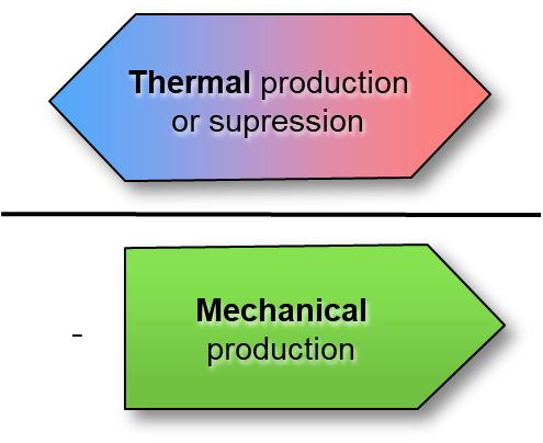
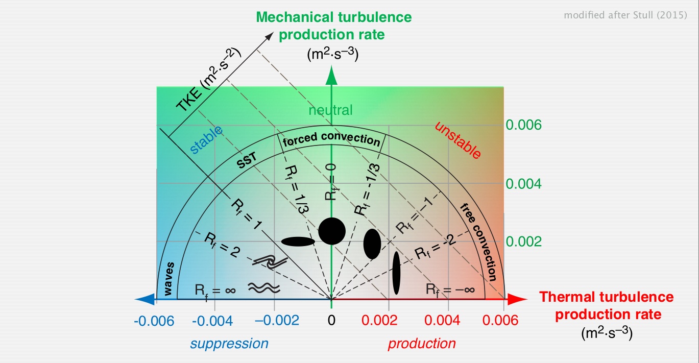
Turbulence Production and Suppression

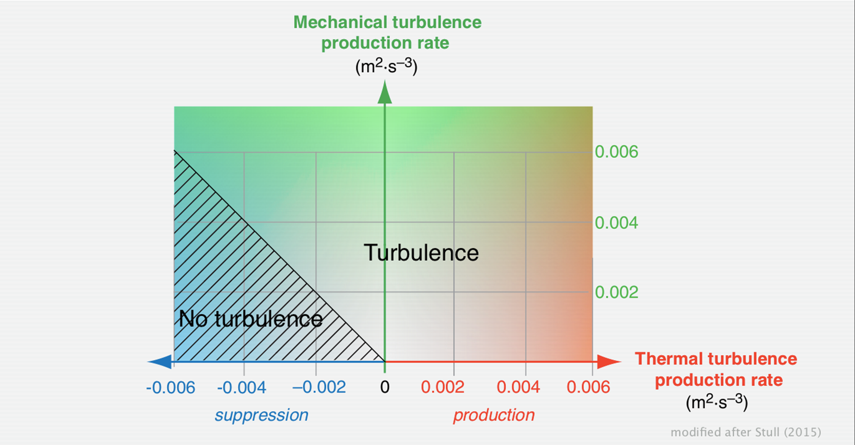
• Mechanical production can be only zero or positive - wind increases with height is linked to momentum transfer in opposite direction.
• Thermal production can be zero, positive or negative.
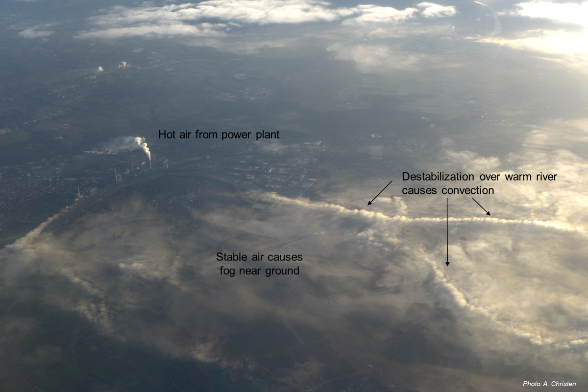
  • A negative thermal production means turbulence suppression, in this case the sensible heat flux cools the atmosphere, increases density, and prevents vertical mixing.

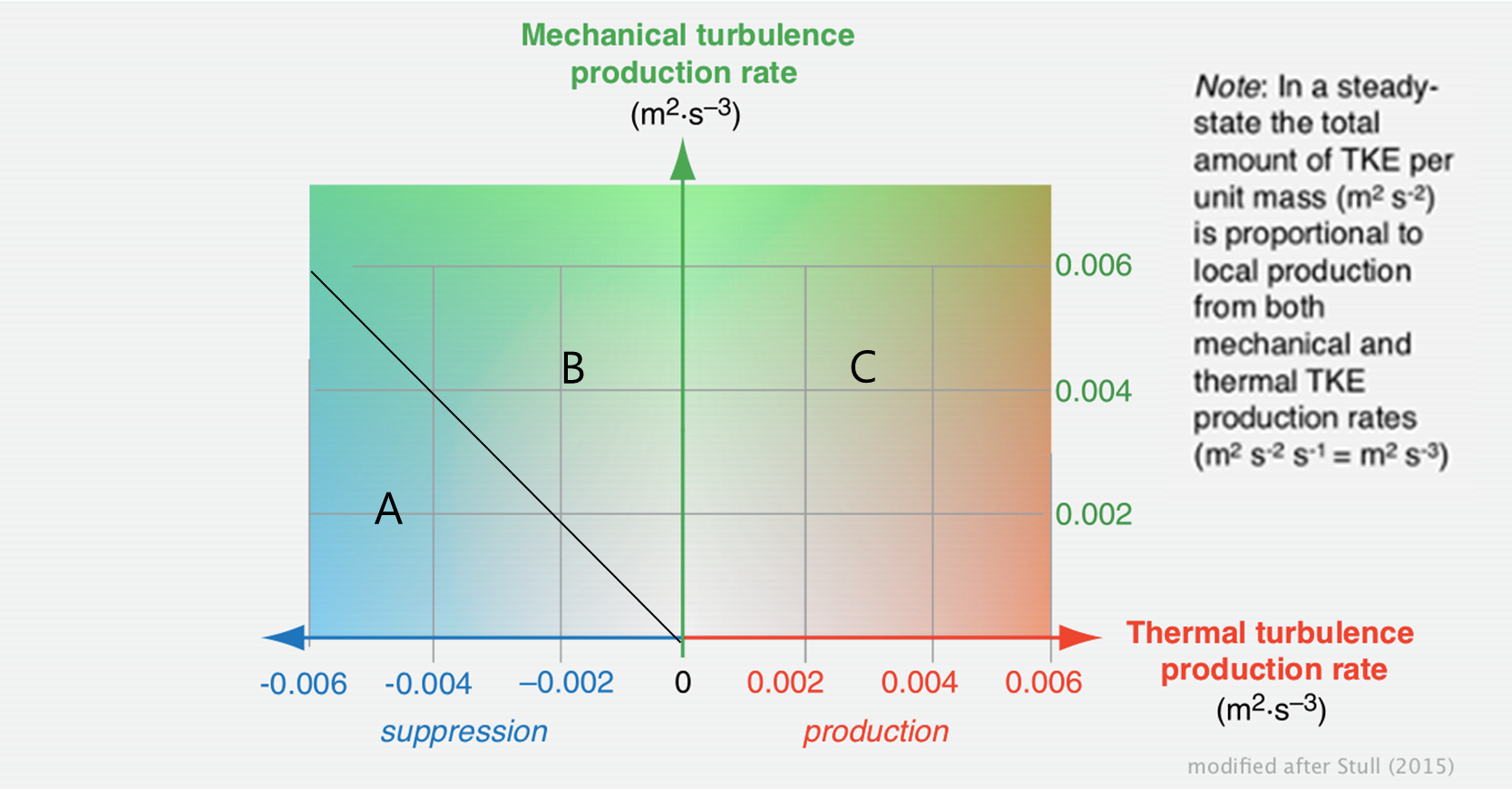
Mechanical vs. Thermal Turbulence

In Steady State, the total amount of TKE per unit mass is proportional to the local production from both mechanical and thermal TKE production rates

TKE < 0

Mechanical vs. Thermal Turbulence

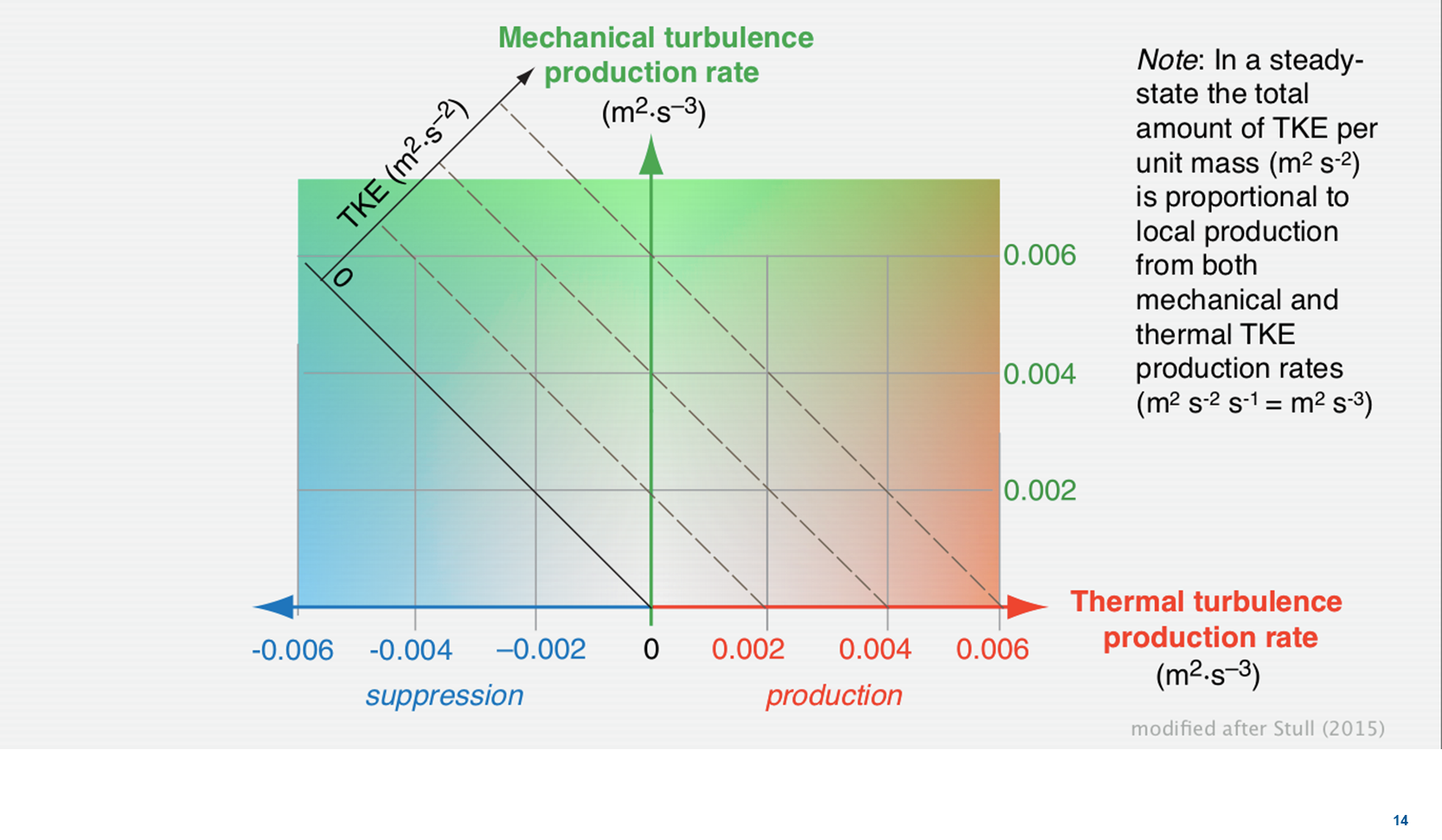
In Steady State, the total amount of TKE per unit mass is proportional to the local production from both mechanical and thermal TKE production rates

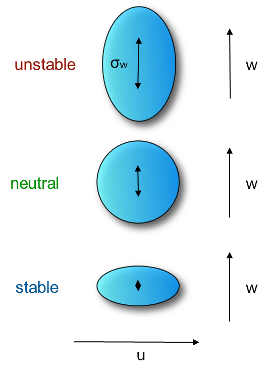
Where will we see no turbulence? (iClicker)

• A: A
• B: B
• C: C
• D: B & C
• E: A, B & C

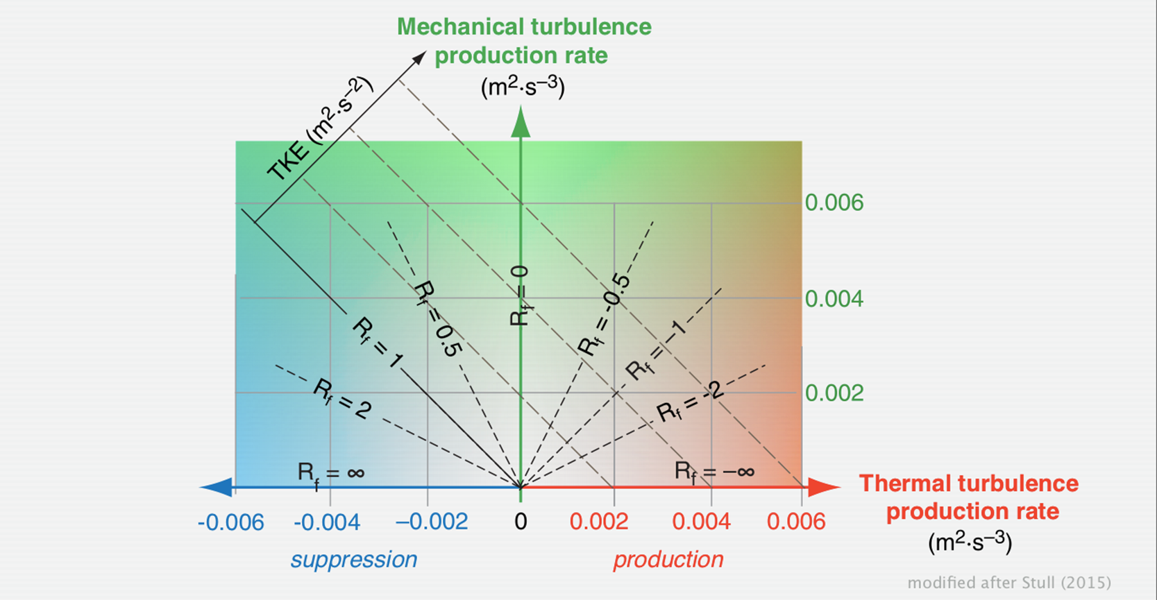
Flux Richardson Number (Rf)

Ratio of the two components gives relative strength of thermal and mechanical production in a flow, expressed by the Flux Richardson number (Rf):

\[ Rf = \frac{\frac{g}{\theta_v}\overline{w^{\prime}\theta_v^{\prime}}}{\overline{u^{\prime}w^{\prime}}\frac{\Delta \bar{u}}{\Delta z}} \qquad(5)\]

• \(Rf\) is a non-dimensional number saying which term is dominant
  • \(Rf\) > 0 : stable
  • \(Rf\) ≈ 0 : neutral
  • \(Rf\) < 0 : unstable

Simply, you can think of \(Rf\) as the ratio of thermal and mechanical componenets

Stable w’T’ < 0 Unstable w’T’ > 0 Neutral w’T’ = 0 Denominator is negative Ri relates the relative roles of buoyancy (numerator) to mechanical (denominator) forces. Good indicator of buoyancy Neutral conditions are the exception rather than the rule in the atmosphere. Neutral conditions where buoyancy is unimportant. Such conditions are found with cloudy skies and strong winds, and in the lowest 1 to 2 m of the atmosphere. Cloud reduces radiative heating and cooling of the surface; strong winds promote mixing and do not permit strong temperature stratification to develop; and in the lowest layers forced convection due to frictionally-generated eddies is dominant.

Flux Richardson Number (Rf)

Stable atmosphere where thermal suppression of turbulence dominates Unstable atmosphere where thermal production of turbulence dominates

Gradient Richardson Number (Ri)

Covariances can be difficult to obtain, so assuming similarity, i.e. \(K_M \approx K_H\), we get the Gradient Richardson number (Ri):

\[ \begin{align} &Rf = \frac{K_H}{K_M} Ri \\ \nonumber &Ri = \frac{g}{\bar{\theta_v}}\frac{\bar{\theta_v}/\Delta z}{(\bar{u}/\Delta z)^2} \end{align} \qquad(6)\]

Instead of Flux Richardson Number (Rf)

Dynamic stability regimes

Table 1: The Flux Richardson number (Rf) is a non-dimensional number that indicate the relative ratio of processes in the production or suppression of turbulence

Rf or Ri	Turbulence regime
Rf < -1/3	free convection
-1/3 < Rf < 1/3	forced convection
1/3 < Rf < 1	stably stratified turbulence (SST)
Rf > 1	no turbulence, only waves

Stable atmosphere where thermal suppression of turbulence dominates Unstable atmosphere where thermal production of turbulence dominates For Rf < 0, unstable atmosphere where we have free convection (the numerator even contributes to the generation of turbulence.) At any value of Rf < +1, static stability is insufficiently strong to prevent the mechanical generation of turbulence. The flow is turbulent (dynamically unstable) when Rf < +1 The flow becomes laminar (dynamically stable) when Rf > +1.

In a statically stable environment, turbulent vertical motions are acting against the restoring force of gravity. Thus, buoyancy tends to suppress turbulence, while wind shears tend to generate turbulence mechanically. The buoyant production term (Term 1lI) of the TKE budget equation (5.1b) is negative in this situation, while the mechanical production term (Term IV) is positive.

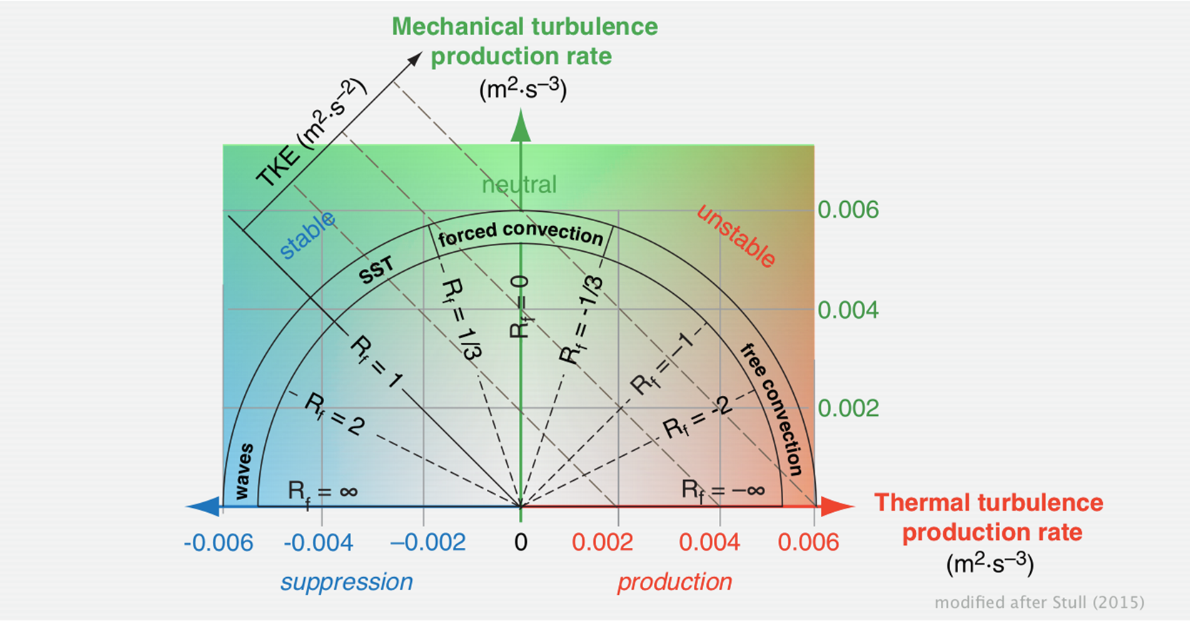
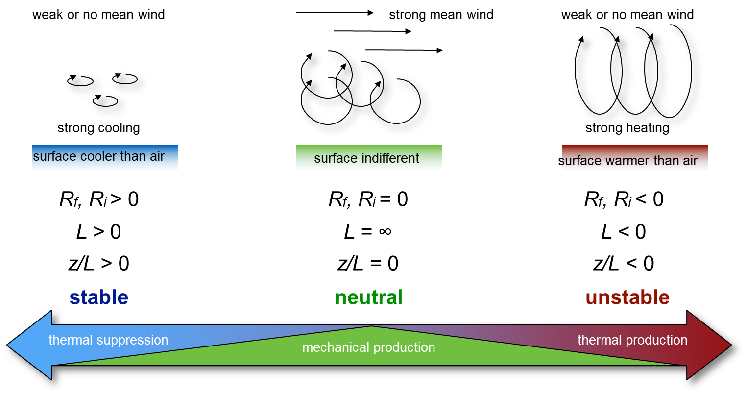
Turbulence regimes in graph of production / suppression

forced convection. These conditions are typical of windy overcast days, and are associated with near neutral static stability When B is positive and |B| > |3·S|, the atmosphere is said to be in a state of free convection. thermals of warm rising air are typical in this situation, and the ABL is statically unstable. These conditions often happen in the daytime over land, and during periods of cold-air advection over warmer surfaces. For B negative but |B| < |S|, weak turbulence is possible. These conditions can occur at night. This is sometimes called stably-stratified turbulence (sst). When B is negative and |B| > |S|, static stability is so strong that turbulence cannot exist. Buoyancy waves (gravity waves) are possible, and appear as waves in the smoke plumes. For values of |B| ≈ |S|, breaking Kelvin-helmholtz waves can occur (see the Stability chapter), which cause some dispersion. When statically stable laminar flow is just becoming dynamically unstable due to an increase in wind shear, the dynamically unstable layer behaves like breaking ocean waves (Fig. 5.17) in slow motion. These waves are called Kelvin-helmholtz waves, or K-h waves for short.

Monin-Obukhov Similarity Theory

\(Rf\) has the disadvantage that it is a function of \(z\) in the ABL. So we are interested in another stability parameter which is not; the “global” dimensionless stability parameter \(\zeta\):

\[ \begin{align} & \zeta = \frac{z}{L} \\ \nonumber & L = - \frac{\bar{\theta_v} u_*^3}{kg\overline{w^{\prime}\theta_v^{\prime}}} = - \frac{\bar{\rho c_a \theta_v} u_*^3}{kgH} \end{align} \qquad(7)\]

Because both friction velocity \(u_*\) and sensible heat flux \(H\) are roughly constant with height near the surface, \(L\) is also invariant with height.

Buoyant production and mechanical production both change in magnitude with height throughout BL, especially mechanical production, so Rf is a function of height. The influence of buoyancy normally increases with higher, at least through the depth of the surface layer, and this is reflected by the fact that the Rf numbers usually increase in magnitude with height. The problem with these stability parameters is that they do not show the effect of height explicitly. Most current boundary layer theory related the structure of the atmosphere to the parameter z/L, where L is the M-O, which shows the variation with height directly.

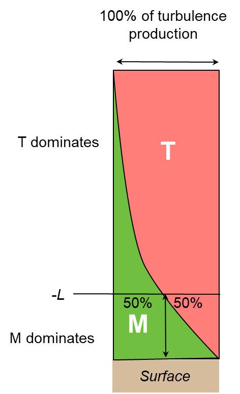
Interpretation of the Obukhov-Length

• Very close to the surface, mechanical production (M) dominates. In the upper ABL typically thermal production dominates (T) because wind shear (\(\Delta u/ \Delta z\)) decreases more rapidly with height than the sensible heat flux (\(w^{\prime}T^{\prime}\)). So there must be a height where M = T.
  • \(L\) can be physically interpreted as the inverse of the height above ground where the mechanical and thermal production are equal, in non-neutral conditions.
  • The sign of \(L\) is given by that of \(H\) and it is related to \(Rf\)

Near the surface, turbulence generated as the wind flows over an aerodynamically rough surface is most important, but higher in the atmosphere convectively generated turbulence tends to dominate. The Obukhov length can be interpreted as the height in the stable surface layer below which shear production of turbulence exceeds buoyant consumption.

Summary of Stability Parameters

Obukhov-Length Zeta

Effect on Eddy Size & Shape

Thus, if turbulence is isotropic, then a smoke puff would tend to expand isotropically, as a sphere; namely, it would expand equally in all directions. There are many situations where turbulence is anisotropic (not isotropic). During the daytime over bare land, rising thermals create stronger vertical motions than horizontal. Hence, a smoke puff would loop up and down and disperse more in the vertical. At night, vertical motions are very weak, while horizontal motions can be larger. This causes smoke puffs to fan out horizontally at night, and for other stable cases. NOTE: v = lateral velocity variances Similar effects operate on smoke plumes formed from continuous emissions. For this situation, only the vertical and are rele- vant. Fig. 19.2 illustrates how isotropy and anisot- ropy affect average smoke plume cross sections.

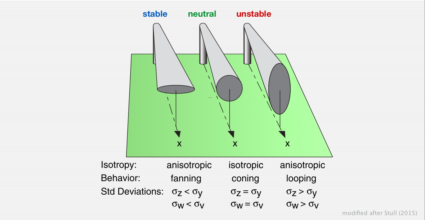
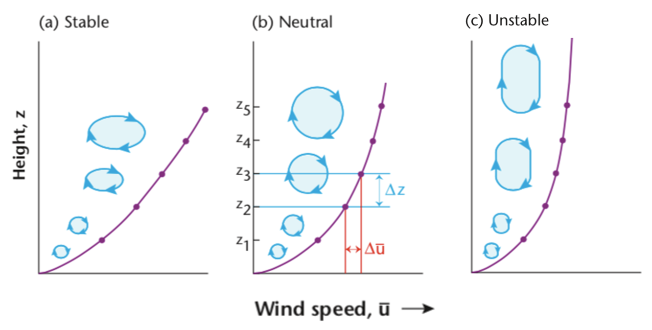
Effect on Eddy Size & Shape

rising thermals create stronger vertical motions than horizontal. vertical motions are very weak, while horizontal motions can be larger

Stability Effects on Profiles and Fluxes

In the neutral case we envisaged eddies as spherical (diameter given by mixing length, \(l = k z\)) and rotating and tangential velocity: \(w^{\prime} = u^{\prime} = u_* = l\frac{\Delta\bar{u}}{\Delta z}\)

• Buoyancy can enhance or diminish vertical motion, so:

• \(w^{\prime} = u^{\prime} \pm \rm{buoyancy}\)

  • Where \(u^{\prime} = l\frac{\Delta\bar{u}}{\Delta z}\) but now \(l\neq k z\)

During the daytime over bare land, rising thermals create stronger vertical motions than horizontal. At night, vertical motions are very weak, while horizontal motions can be larger

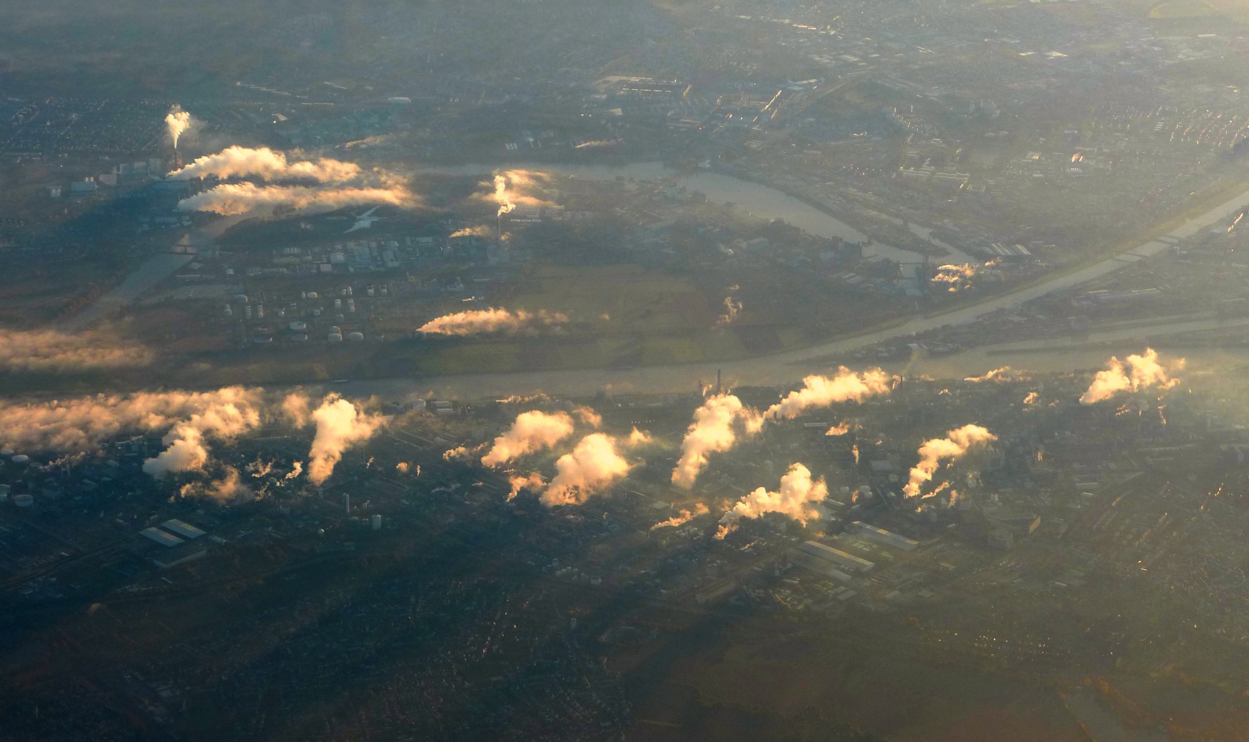
Dispersion of plumes over an industrial area

Photo: A. Christen

At night, vertical motions are very weak, while horizontal motions can be larger Fan out horizontally at night, and for other stable cases.

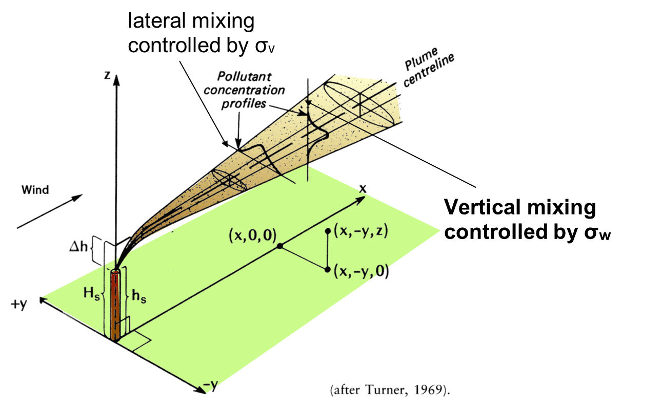
Why is σw/u* of importance?

Relevant to estimate spread of pollutants During the daytime over bare land, rising thermals create stronger vertical motions than horizontal. Hence, a smoke puff would loop up and down and disperse more in the vertical. At night, vertical motions are very weak, while horizontal motions can be larger. This causes smoke puffs to fan out horizontally at night, and for other stable cases.

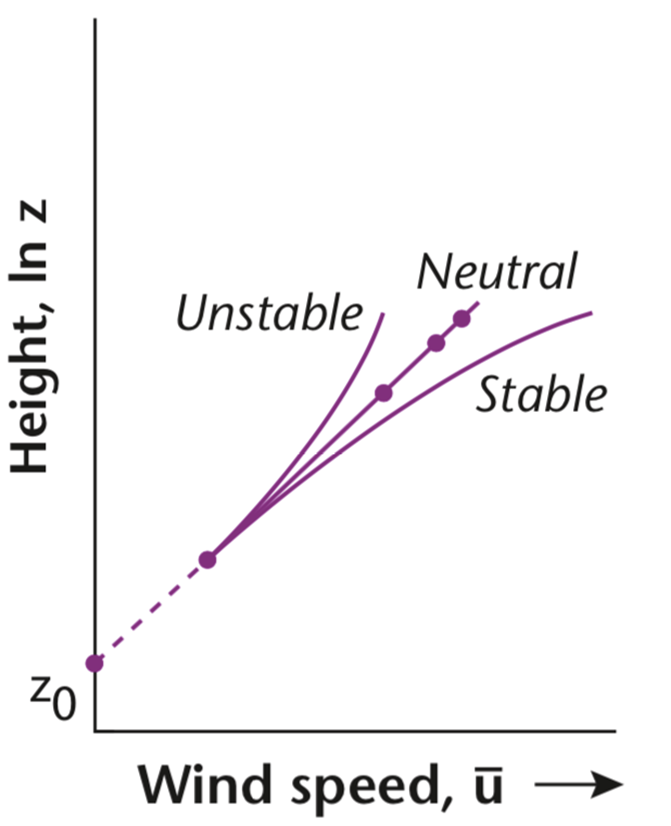
Modification of the wind profile with changing stability

Neutral: The foregoing discussion relates to neutral conditions where buoyancy is unimportant. Such conditions are found with cloudy skies and strong winds, and in the lowest 1 to 2 m of the atmosphere. In the simplest interpretation these eddies may be conceived as being circular and to increase in diameter with height (Figure 2b). In reality they are three-dimensional and comprise a wide variety of sizes. In unstable conditions the vertical movement of eddies is enhanced. Near the surface mechanical effects continue to dominate but at greater heights thermal effects become increasingly more important. This results in a progressive vertical stretching of the eddies and a reduction of the wind gradient (Figure 2a). Conversely strong stability dampens vertical movement, progressively compresses the eddies and steepens the wind gradient (Figure 2c).

Stability effects on wind profile

We need a way of ‘correcting’ the neutral form of the wind profile law to include non-neutral situations:

\[ \frac{\Delta\bar{u_z}}{\Delta z}=\frac{u_*}{k}\Phi_M \qquad(8)\]

where \(\Phi_M\) is a stability correction that can be approximated as:

\[ \Phi_M = \begin{cases} \zeta > 0 , 1 + 4.7 \zeta \\ \zeta = 0 , 1 \\ \zeta < 0 , (1 - 15 \zeta)^{-0.25} \end{cases} \qquad(9)\]

An idealized vertical profile of the mean flow for a neutral boundary layer is the logarithmic wind profile derived from Prandtl’s mixing length theory,[3] which states that the horizontal component of mean flow is proportional to the logarithm of height. M–O similarity theory further generalizes the mixing length theory in non-neutral conditions by using so-called “universal functions” of dimensionless height to characterize vertical distributions of mean flow and temperature. The Monin-Obukhov Similarity Theory allows us to predict the behavior of wind profiles under stable and unstable conditions. A nondimensional wind velocity gradient can be defined as a function of a non-dimensional height, z/L A thermodynamic change of state of a system in which the system exchanges energy with its surroundings by virtue of a temperature difference between them. There are five categories of diabatic processes: solar and terrestrial radiation, latent and sensible surface heat flux, and friction. Figure 6illustrates how diabatic heating is distributed on the seasonal and zonal means.

Correction factors depend on turbulence regime

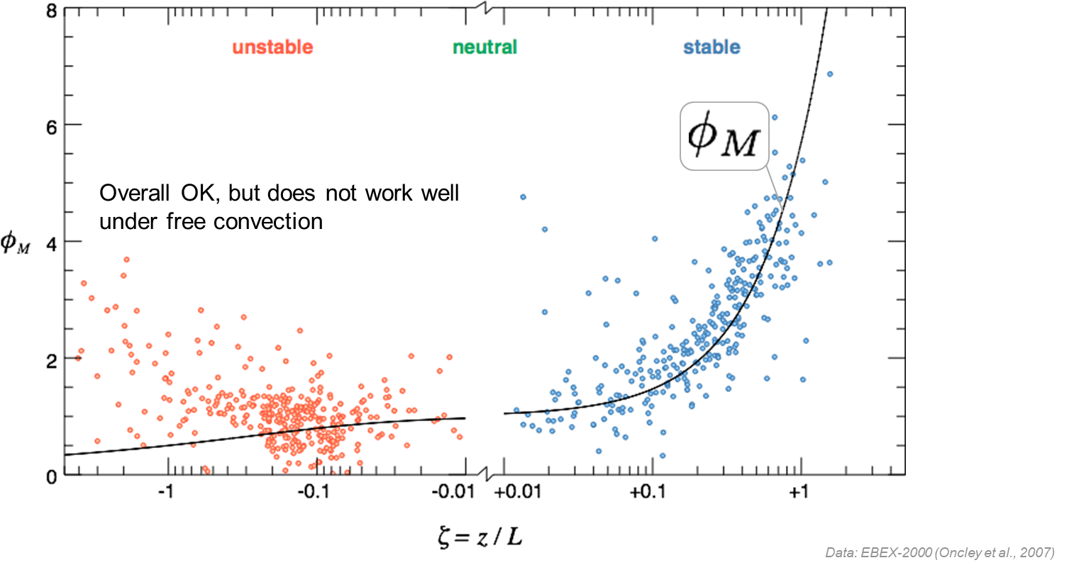
Experimentation across multiple sites allowed us to test the empirical function to approximate \(\Phi_M\). The empirical estimate of \(\Phi_M\) breaks down under strongly unstable conditions.

This example shows data from the same tower you used in assignment #3

A nondimensional wind velocity gradient can be defined as a function of a non-dimensional height, z/L: global dimensionless stability parameter ζ (a greek ‘zeta’) The stability function \(\Phi_M\) is \(\Phi_M\) = 1 in the neutral case \(\Phi_M\) > 1 in stable case \(\Phi_M\) < 1 in the unstable case

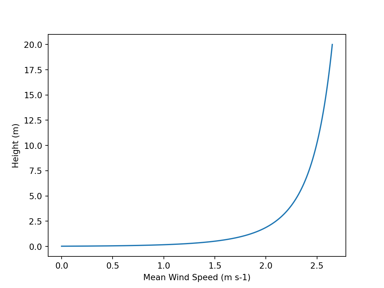
Numerical Integration of Wind Profile

To calculate wind at any height z under diabatic conditions, you must numerically integrate over finite layers, adjusting \(\zeta=z/L\) as you move up (or down).

import numpy as np
def get_Phi_M(zeta):
    Phi_M = np.ones(zeta.shape)
    # Stable/Neutral
    Phi_M[zeta>0] = 1 + 4.7 * zeta[zeta>0]
    # Unstable
    Phi_M[zeta<0] = (1 - 15 * zeta[zeta<0])**-0.25
    return (Phi_M)

def integrate_profile(L,u_star,z0,z,step_size = 0.001):
    k = 0.41
    # Create an array of Z values at "step_size" resolution
    Z = np.arange(z0,z,step_size)
    # Calculate stability parameter
    zeta = Z/L
    # Get zeta values
    Phi_M = get_Phi_M(zeta)
    # Get slope wind profile at each z
    dubar_dz = u_star/(k*Z)*Phi_M
    # Integrate by step, starting at z0 where u_bar = 0
    u_bar = np.cumsum(dubar_dz*step_size)-(dubar_dz[0]*step_size)
    return(Z,u_bar)

L = -10
u_star = 0.2
z0 = 0.02
z = 20

Z,u_bar = integrate_profile(L,u_star,z0,z)
print(Z[-1],u_bar[-1])

19.999000000000017 2.650378708658456

Visualizing the Profile

import matplotlib.pyplot as plt
plt.figure()
plt.plot(u_bar,Z)
plt.ylabel('Height (m)')
plt.xlabel('Mean Wind Speed (m s-1)')
plt.show()

Practical Applications?

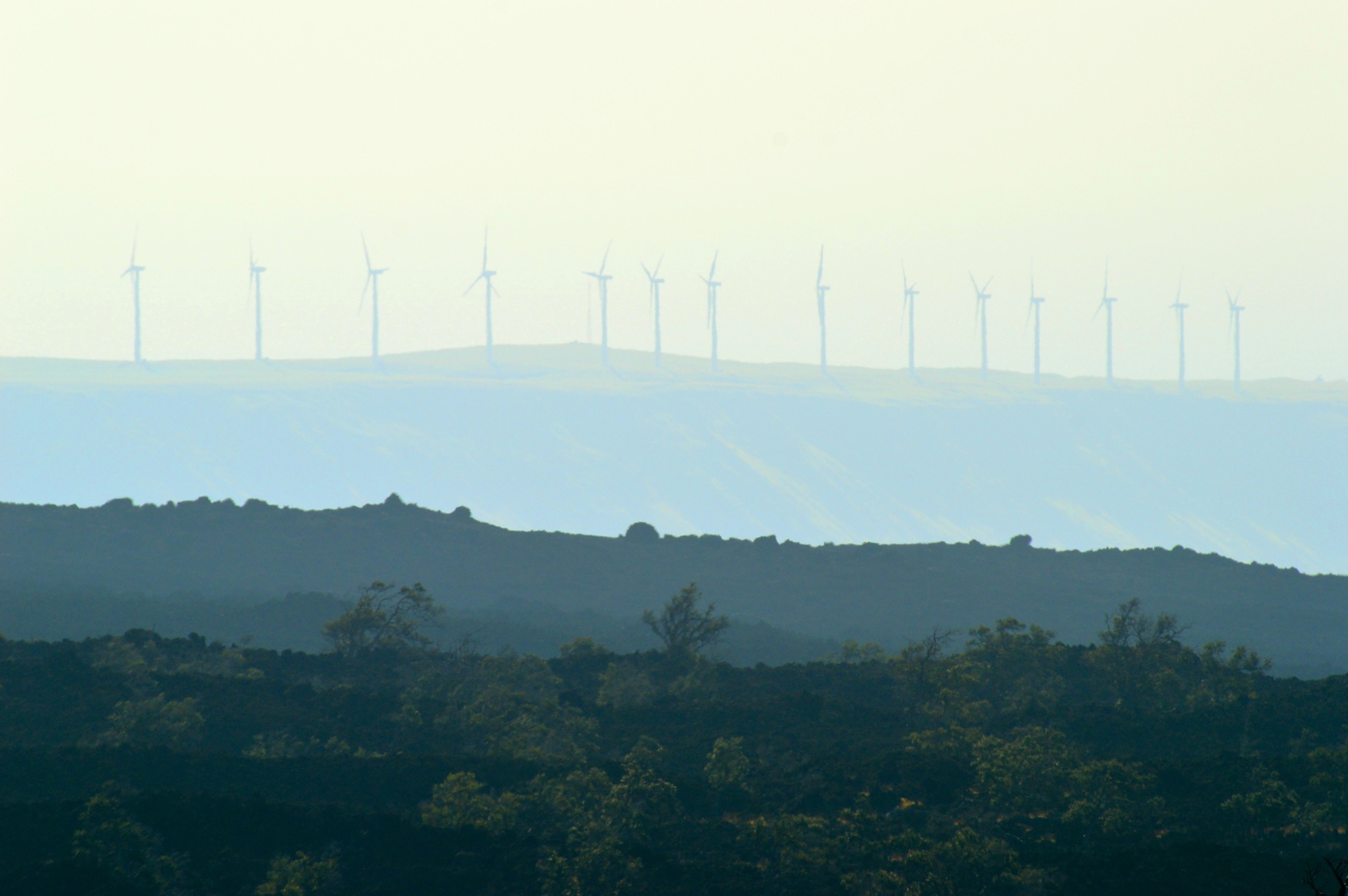
Estimating wind under all conditions is relevant in the wind energy industry (Photo: A. Christen)

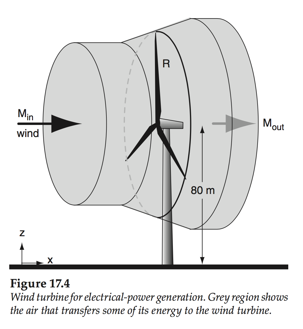
Wind Power Generation

We can estimate the power generation \(U\) (in W) by a wind turbine using the following equation:

\[ U = \frac{\pi}{2}\rho E R^2 \bar{u}^3 \qquad(10)\]

Where \(R\) is the radius of the turbine (in m), \(E\) is the turbine efficiency (usually ~ 30 - 45%), and \(\bar{u}\) is the mean wind speed at the height of the turbine.

Stull R. B. (2015): Practical Meteorology

Write on board!

Example 1

Estimate the power generation of a turbine with \(R\) = 30m, \(z\) = 80m and \(E\) = 40% under the following conditions: Neutral stability, \(u_*\) = 0.5 m/s, \(z_0\) = 0.02 m, \(\rho\) = 1.22 kg m-3:

import numpy as np
k = 0.41
R = 30 # m
E = 0.40 # %
z = 80 # m
z0 = 0.02 # m
u_star = 0.5 # m/s
rho = 1.22 # kg m-3

u_bar = u_star/k *np.log(z/z0)

U = np.pi/2*rho*E*(R**2)*(u_bar**3)

print(f'{U*1e-3:.1f} kW')

713.9 kW

Write log-wind profile Joule: one newton acts on that object in the direction of its motion through a distance of one metre (kg⋅m2⋅s−2) W: 1 joule per second

Example 2

Estimate the power generation of the same turbine if all conditions are the same, except: Unstable (L = -2):

import numpy as np
z0 = 0.02 # m
u_star = 0.5 # m/s
rho = 1.22 # kg m-3
L = -2

# Get integrated profile
Z,u_bar = integrate_profile(L,u_star,z0,z)
# Estiamte U for 
U = np.pi/2*rho*E*(R**2)*(u_bar[-1]**3)
print(f'{U*1e-3:.1f} kW')

134.2 kW

Stability effects on temperature profiles

How do we interpret this? (iClicker)

• A: All else equal unstable conditions enhance wind power generation

• B: All else equal unstable conditions inhibit wind power generation

• C: Not enough information to know?

How did power generation compare between the two conditions?

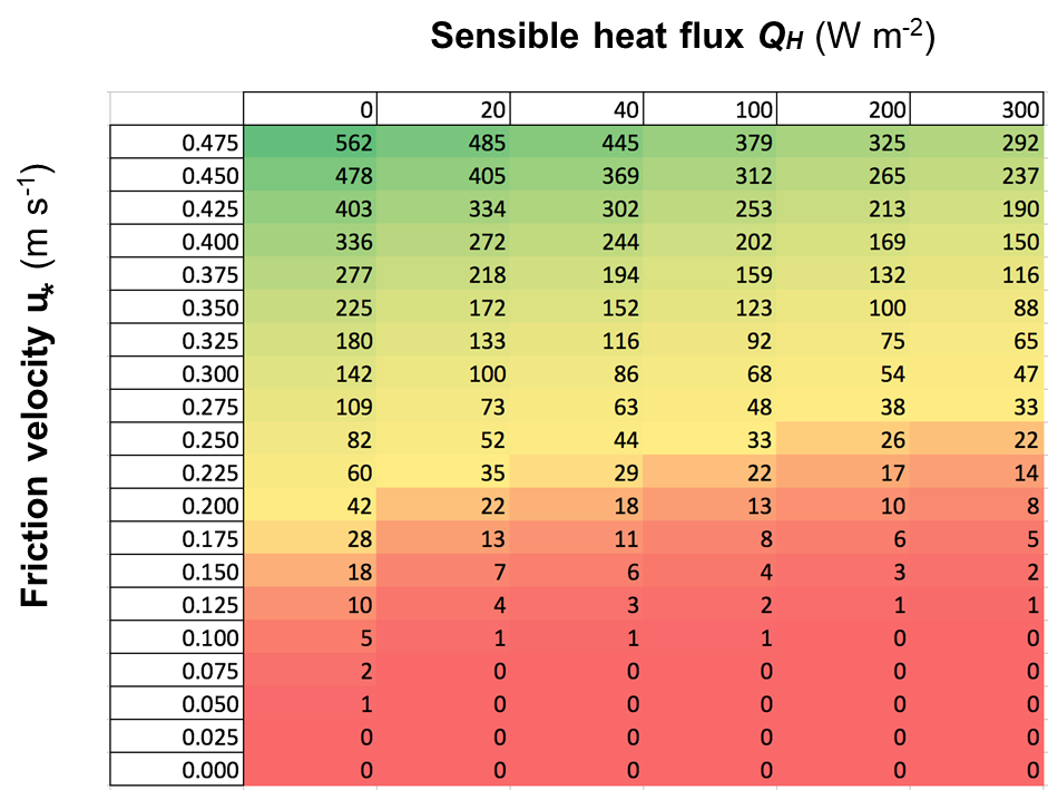
Wind Energy vs. Sensible Heat Flux

Estimate the power generation (kW) of the same turbine

As a consequence the wind gradient becomes weaker under unstable and stronger under stable conditions.

Take home points

• Dynamic stability parameters describe ratio of thermal turbulence production to (minus) mechanical turbulence production.
• Dimensionless flux and gradient Richardson numbers are commonly used to describe the atmosphere’s dynamic stability and the turbulence regime.
• Monin-Okukhov similarity theory (MOST) is using four variables controlling turbulence, u*, w’T’, g and T and derives a stability length L (called the Obukhov length)
• Dynamic stability controls the eddy spectrum and eddy shape.
• Under non-neutral (diabatic) conditions, the mixing length changes, and so does the vertical extent of eddies.
• As a consequence the wind gradient becomes weaker under unstable and stronger under stable conditions.
• A a set of semi-empirical correction functions can be used to predict wind profiles under such conditions.
• Such relations are for example relevant to estimate spread of pollutants or wind energy potential.