Eddy Covariance

Measuring scalar transport via turbulent exchange

Learning Objectives

• Describe the eddy covariance approach & what observations are required to measure flux densities using this approach.
• Describe the equations used to calculate H, LE and trace gas fluxes.
• Be able to interpret eddy covariance observations of Net Ecosystem Exchange (NEE).

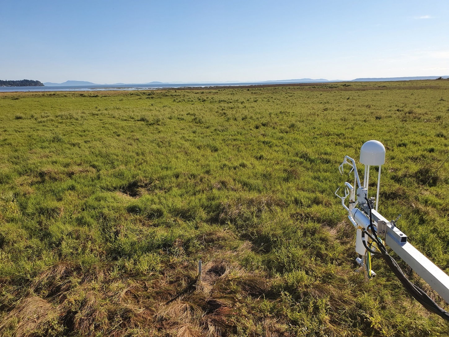
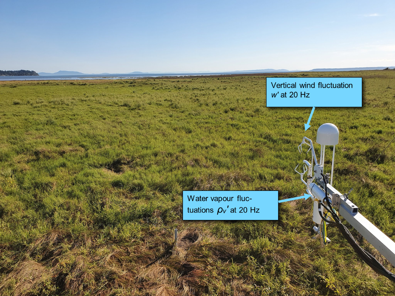
Measurement of convective fluxes using the EC technique at a salt marsh in Boundary Bay, Delta, BC (Photo: Tzu-Yi Lu, UBC)

iClicker

How do you submit the extra credit field trip assignment?

• A: Submit on Canvas as part of Assignment 4
• B: Submit on Canvas in the Final Exam
• C: Email it in anytime before the Final Exam

Convective transport

Turbulence and associated eddies transport not only momentum but also heat and mass.

• Turbulence is the most relevant vertical transport mechanism in the ABL.

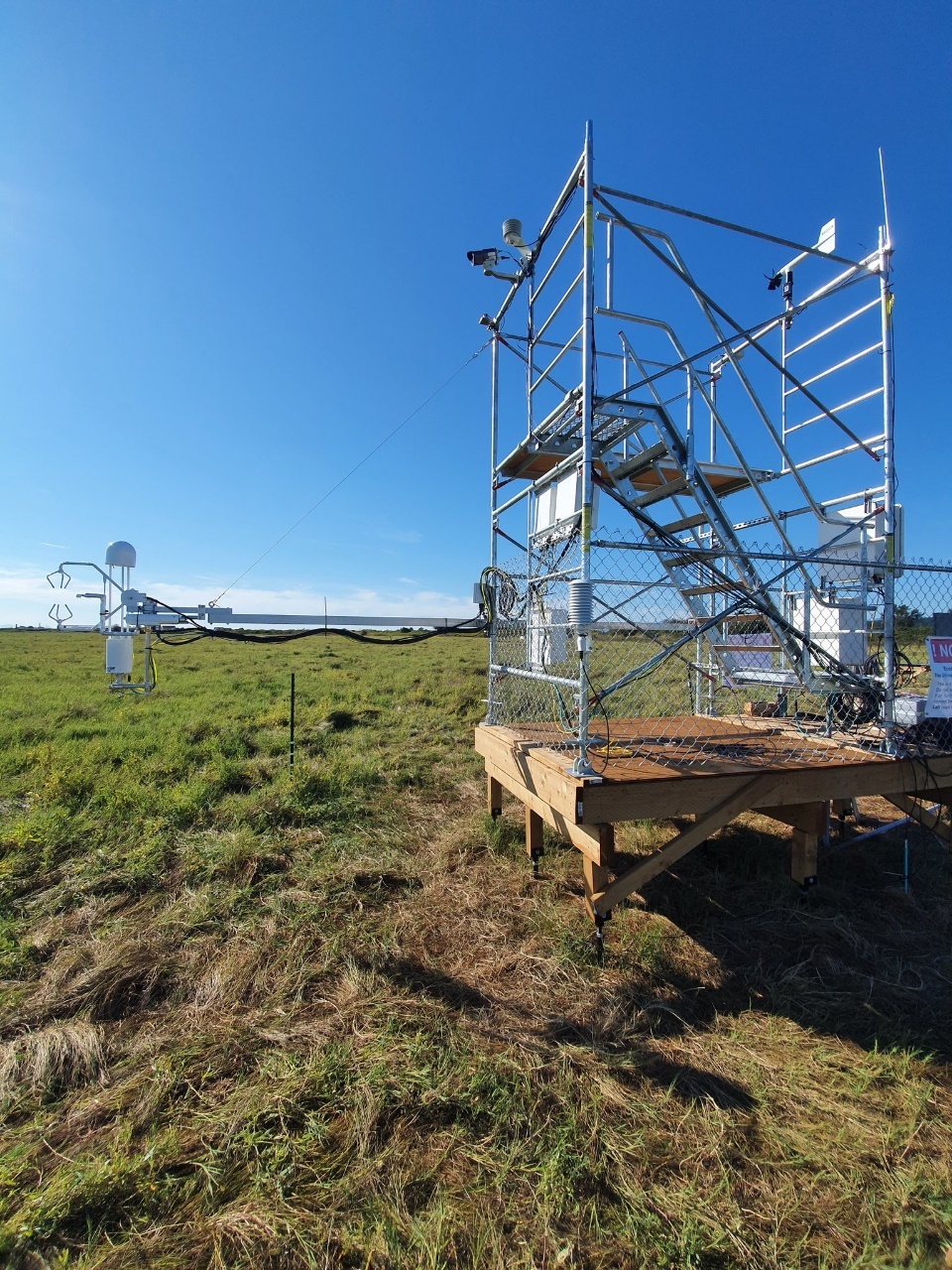
Tower with eddy covariance instrumentation Photo: Nick Lee

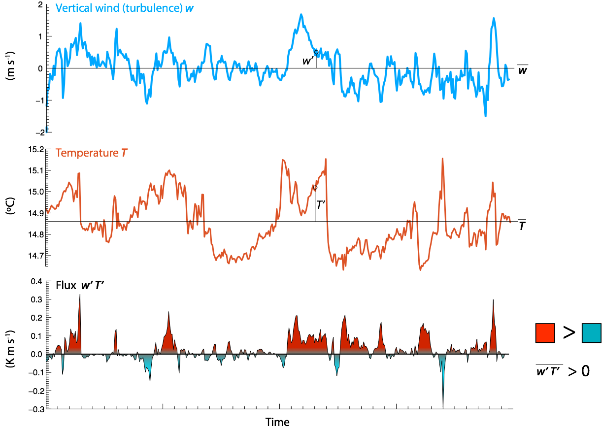
Evidence of Convective Transport in a Time Series

Simultaneous measurements at 6 heights on a tower of wind vector (arrows) and temperature (colors)

Test your knowledge

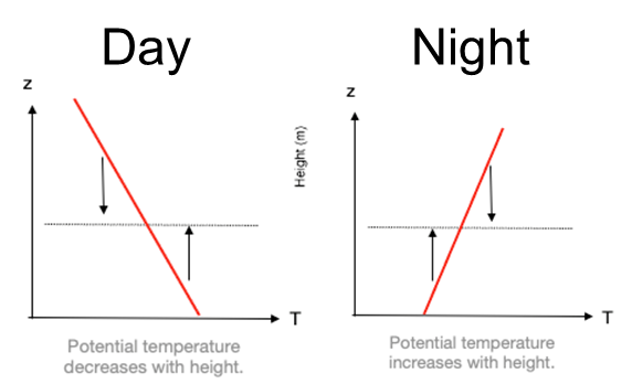
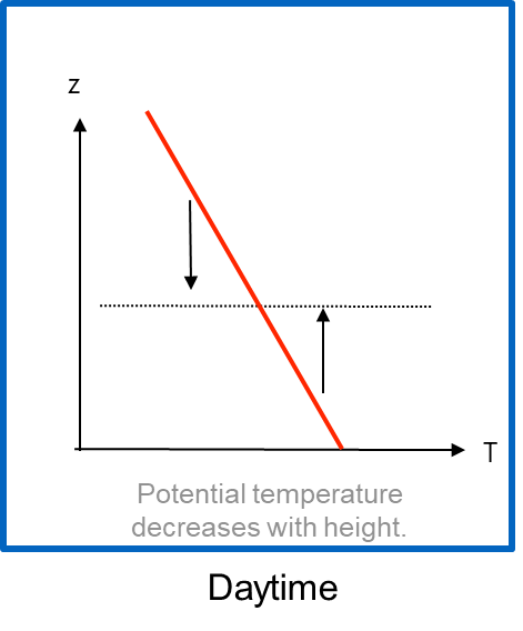
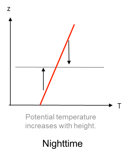
What temperature profile do those observations correspond to? A (daytime) or B (nighttime)

Simultaneous measurements at 6 heights on a tower of wind vector (arrows) and temperature (colors)

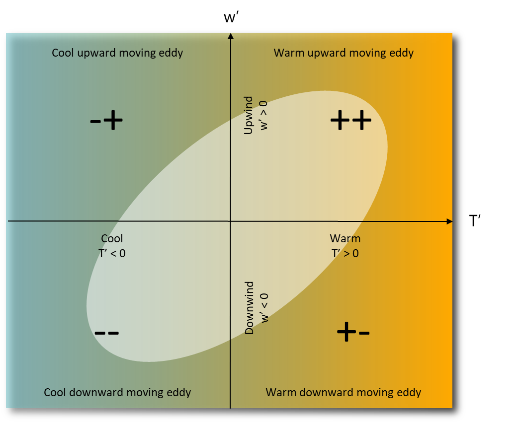
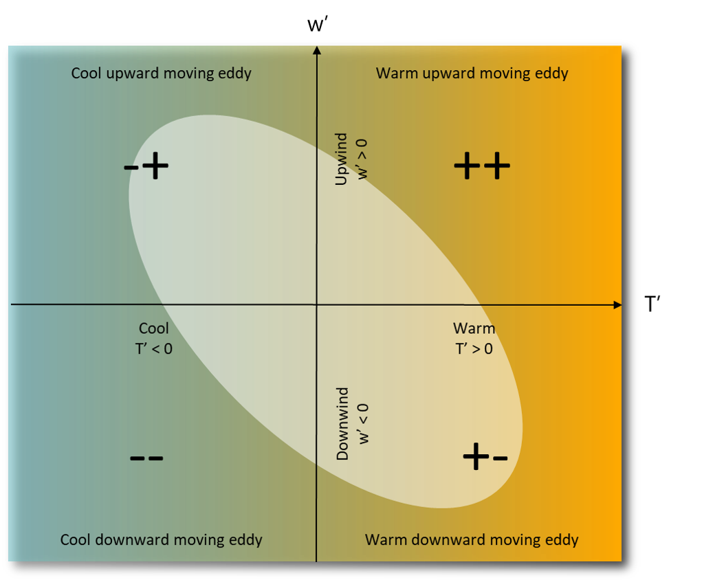
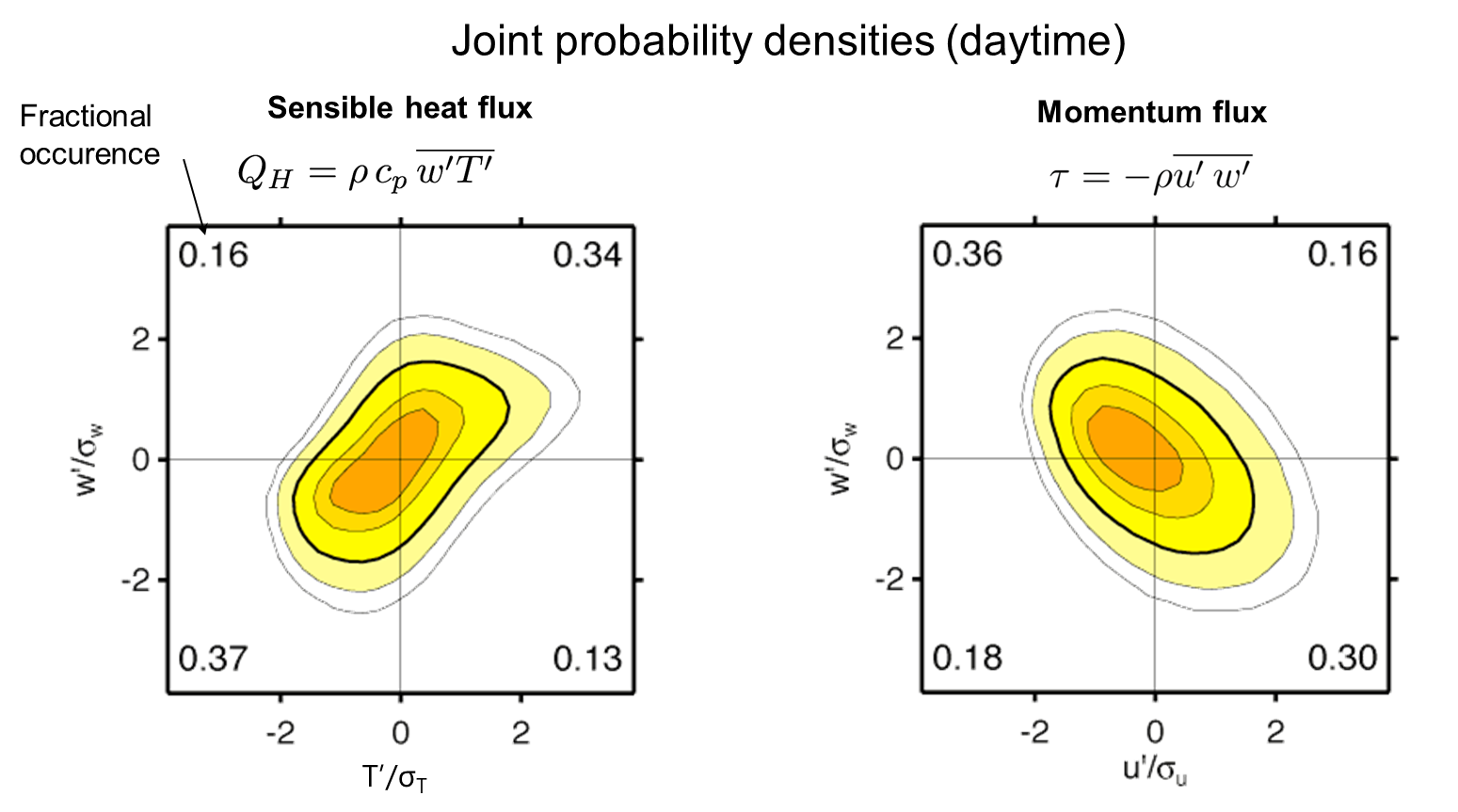
Daytime Joint PDF \(w^{\prime} T^{\prime}\)

Sensible heat flux transports energy away from the surface: \(\overline{w^{\prime}T^{\prime}} > 0\)

Fast Trace of Signals

Figure 2 very clearly illustrates how the product of w’ and T’ combine to produce an instantaneous sensible heat flux (QH ). The time average of this heat flux is the value given by equation

Nighttime Joint PDF \(w^{\prime} T^{\prime}\)

Sensible heat flux transports energy towards from the surface: \(\overline{w^{\prime}T^{\prime}} < 0\)

Turbulence is the most relevant vertical transport mechanism in the ABL.

Covariance and flux densities (1/2)

The vertical flux density of an entity \(c\) is defined as:

• Flux density (amount of c \(m^{-2} s^{-1}\)) = air density (\(kg\ m^{-3}\)) \(\times\) vertical velocity (\(m s^{-1}\)) \(\times\) the amount of c (units vary)

• For some entity \(c\), the general form for average flux density is:

\[ F_c = \overline{\rho w c } \qquad(1)\]

Recall: applying Reynolds decomposition to each component:

\[ \begin{align} \rho=\bar{\rho}+\rho^{\prime} \\ \nonumber w=\bar{w}+w^{\prime} \\ \nonumber c=\bar{c}+c^{\prime} \\ \nonumber \end{align} \]

The theory behind these measurements. The eddy covariance method is based on the turbulent transport theory in the surface layer of the atmosphere and used to estimate scalar and energy fluxes from the covariance between the vertical wind speed and the gas concentration at a measured height above the surface.

All atmospheric entities show short-period fluctuations about their longer term mean value. This is the result of turbulence which causes eddies to move continually around carrying with them their properties derived elsewhere.

Extensive site mass continuity requires that as much air moves up as moves down over a reasonable period of time (e.g. 10 min); and the detail of the fluctuating trace gives the value of w0 at any instant as a positive or negative quantity depending upon whether it is above the mean (an updraft) or below it (a downdraft).

The properties contained by, and therefore transported with, an eddy are its mass (which by considering unit volume is given by its density, (⇢), its vertical velocity (w) and the volumetric content of any entity it possesses (s). Since each one can be broken into a mean and a fluctuating part the mean vertical flux density of the entity (S) can therefore be written

Covariance and flux densities (2/2)

Close to the surface, \(\bar{w} \rightarrow 0\) and \(\rho^{\prime} \approx 0\), therefore, Equation 1 reduces to:

\[ F_c = \overline{\bar{\rho}w^{\prime}(\bar{c}+c^{\prime})} = \overline{\bar{\rho}(w^{\prime}\bar{c}+w^{\prime}c^{\prime})} \nonumber \]

Recalling that \(\overline{\bar{c}\times w^{\prime}} =0\); a flux density can be expressed in terms of the correlation coefficient:

\[ F_c = \rho \overline{w^{\prime}c^{\prime}} \qquad(2)\]

First, all terms involving a single primed quantity are eliminated because by definition the average of all their fluctuations equals zero (i.e. we lose the second, third and fifth terms). Second, we may neglect terms involving fluctuations of density since air density is considered to be virtually constant in the lower atmosphere (i.e. we lose the sixth, seventh and eighth terms. Third, if observations are restricted to uniform terrain without areas of preferred vertical motion (i.e. no ‘hotspots’ or standing waves) we may neglect terms containing the mean vertical velocity, as w = 0 (i.e. we lose also the first term). With these assumptions equation 9.26 reduces to the form of the relation underlying the eddy fluctuation approach. Redefine correlation coefficient Flux = turbulent fluctuations in vertical wind and the scalar, and then computing the covariance between the two.

A Helpful Explanation

Measuring Sensible Heat Flux Density H by EC

The instantaneous sensible heat flux density is (in W m-2):

\[ H = C_a w^{\prime}T^{\prime} \nonumber \qquad(3)\]

Averaging and substituting \(\rho c_a\) gives:

\[ H = \rho c_a \overline{w^{\prime}T^{\prime}} \qquad(4)\]

Specific heat: kJ kg-1 K-1

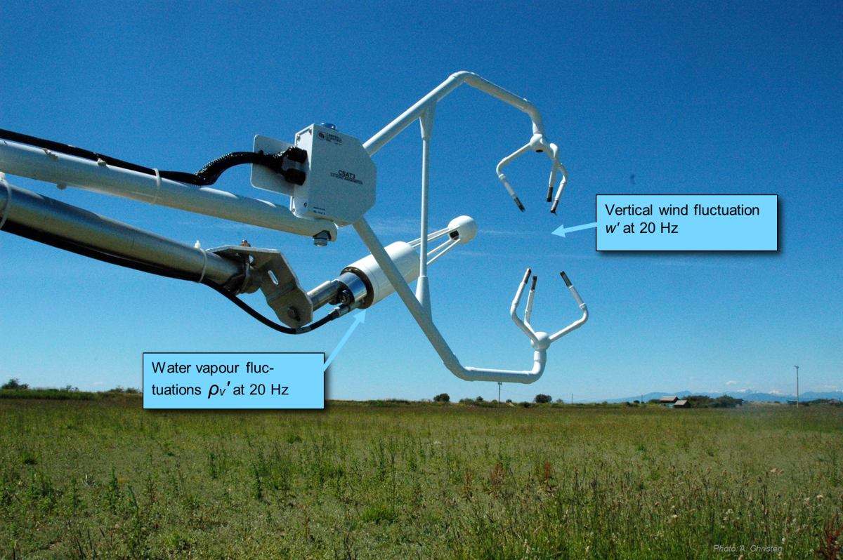
A Typical Setup

A Typical Setup

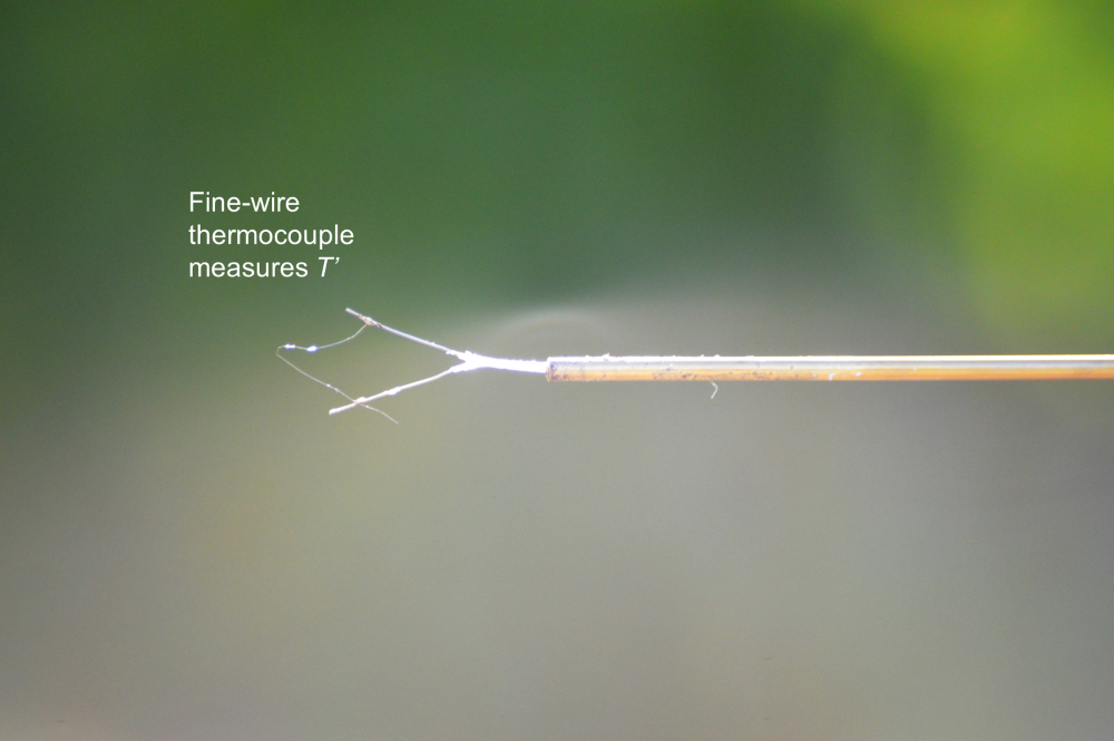
Fast Response Temperature

Sensible heat flux vs. momentum flux

Sensible heat flux vs. momentum flux (iClicker)

Which (if either) of these joint probability distributions would you expect to have an inverted relationship at nighttime?

• A Sensible Heat Flux
• B Momentum Flux
• C Both
• D Neither

Because u is increasing with height, the horizontal momentum flux is negative throughout the boundary layer. 

Latent heat flux density LE

The instantaneous latent heat flux density is (in W m-2):

\[ LE = L_v w^{\prime}\rho_v^{\prime} \nonumber \qquad(5)\]

Where \(\rho_v\) is the partial vapor density of water (aka absolute humidity) and \(L_v\) is the latent heat of vaporization in \(J \ kg^{-1}\) (see next slide). Averaging gives:

\[ LE = L_v \overline{w^{\prime}\rho_v^{\prime}} \qquad(6)\]

measure mole density, not mixing ratio

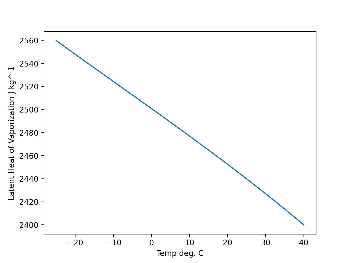
Latent Heat of Vaporization

Following Yao & Rogers (1996), the latent heat of vaporization of water (\(L_v\) in \(J g^{-1}\)) can be approximated as a function of temperature (\(T\) in \(^{\circ}C\)) using a third order polynomial function:

\[ L_v = 2500.8-2.36T-0.0016T^2-0.00006T^3 \qquad(7)\]

While \(L_v\) varies as a function of \(T\); over small temperature ranges, the differences are negligible

A Typical Setup

A Typical Setup

Mass trace gas flux

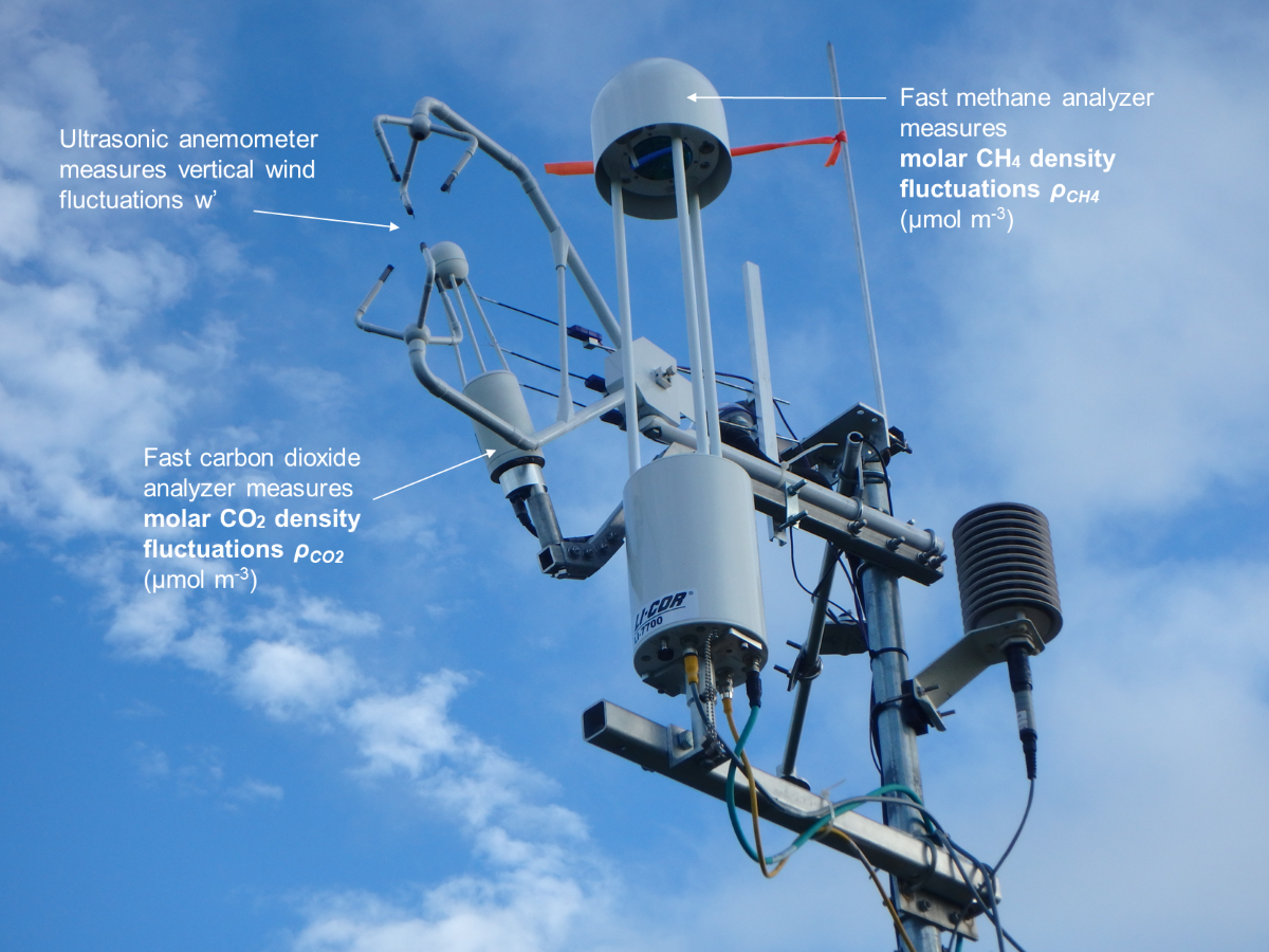
If we equip an eddy covariance system with an analyzer that measures fast fluctuations of the molar density of any trace gas \(\rho_c^{\prime}\) (e.g. µmol m-3) we can directly determine the gas-exchange (molar flux) between a land surface and the atmosphere:

\[ F_c = \overline{w^{\prime}\rho_c^{\prime}} \qquad(8)\]

To convert a molar trace gas flux to a mass flux, you multiply by the molar mass M (\(\rm{g} \ \rm{mol}^{-1}\)) of the compound. For example the molar mass of \(\rm{CO}_2\) is 44.01 \(\rm{g} \ \rm{mol}^{-1}\)

A Typical Setup

Measuring the ‘breathing’ of our biosphere

Net Ecosystem Exchange (of CO₂) and Latent Heat (Energy) Fluxes over a year at a salt marsh in Delta, BC

Net Ecosystem Exchange

Fluxes of carbon dioxide (CO₂) are of particular concern for micrometeorologists, climate scientists, and ecologists because of the role ecosystem-scale CO₂ exchange plays in the global climate system.

• Measurements of Net Ecosystem Exchange (NEE) are an important component of monitoring the effects of an predicting the progression of climate change!

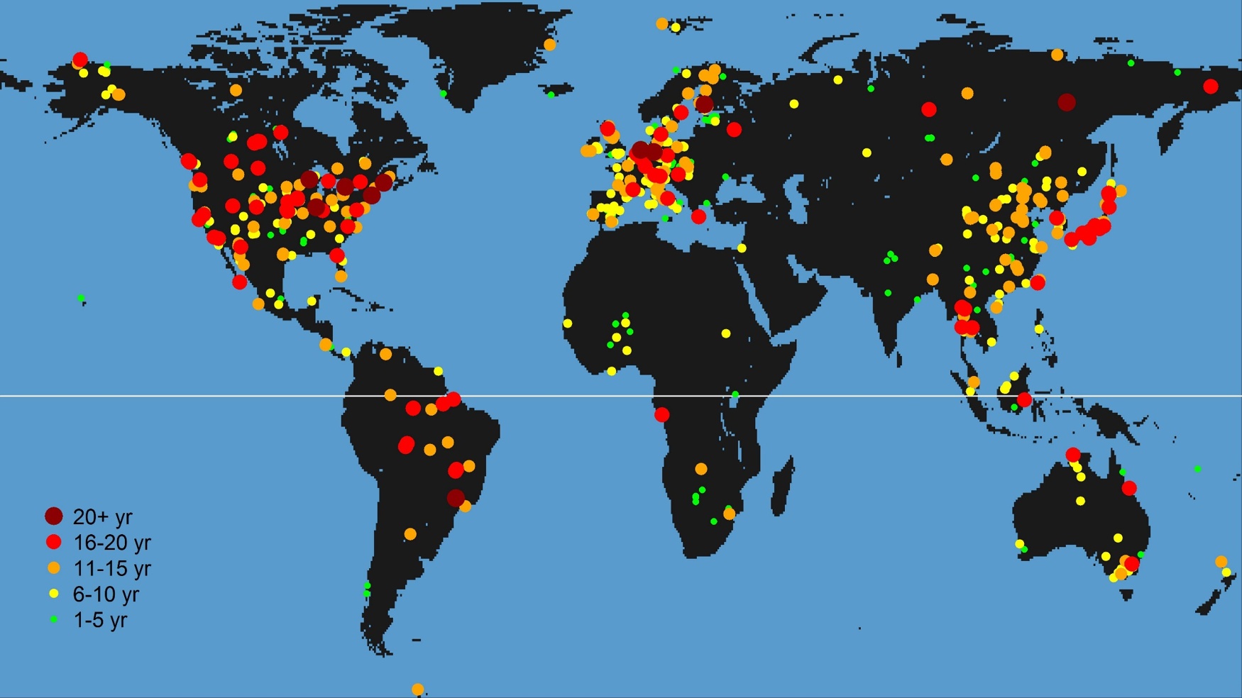
FLUXNET – a global network of EC sites

Source: http://fluxnet.fluxdata.org/

1. Go to: https://ameriflux.shinyapps.io/version1/

2. Select site US-Ha1 & plot CO2_1_1_1 (CO2 concentration) as the Y-axis variable What do you see?
3. Now change the Y-axis variable to FC_1_1_1 What do you observe?
4. Click on ‘All Sites’ & change the Y-axis variable to ‘NEE’
5. Create your own plot(s)

Visualizing eddy covariance data (30 min avg data)

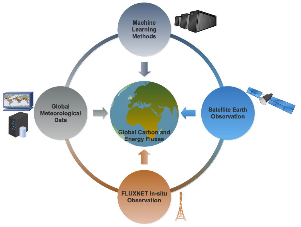
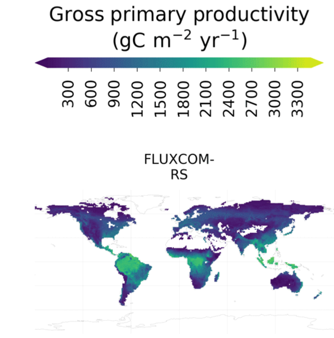
Research example – upscaling EC to the global scale

Jung et al. 2020 Biogeosciences

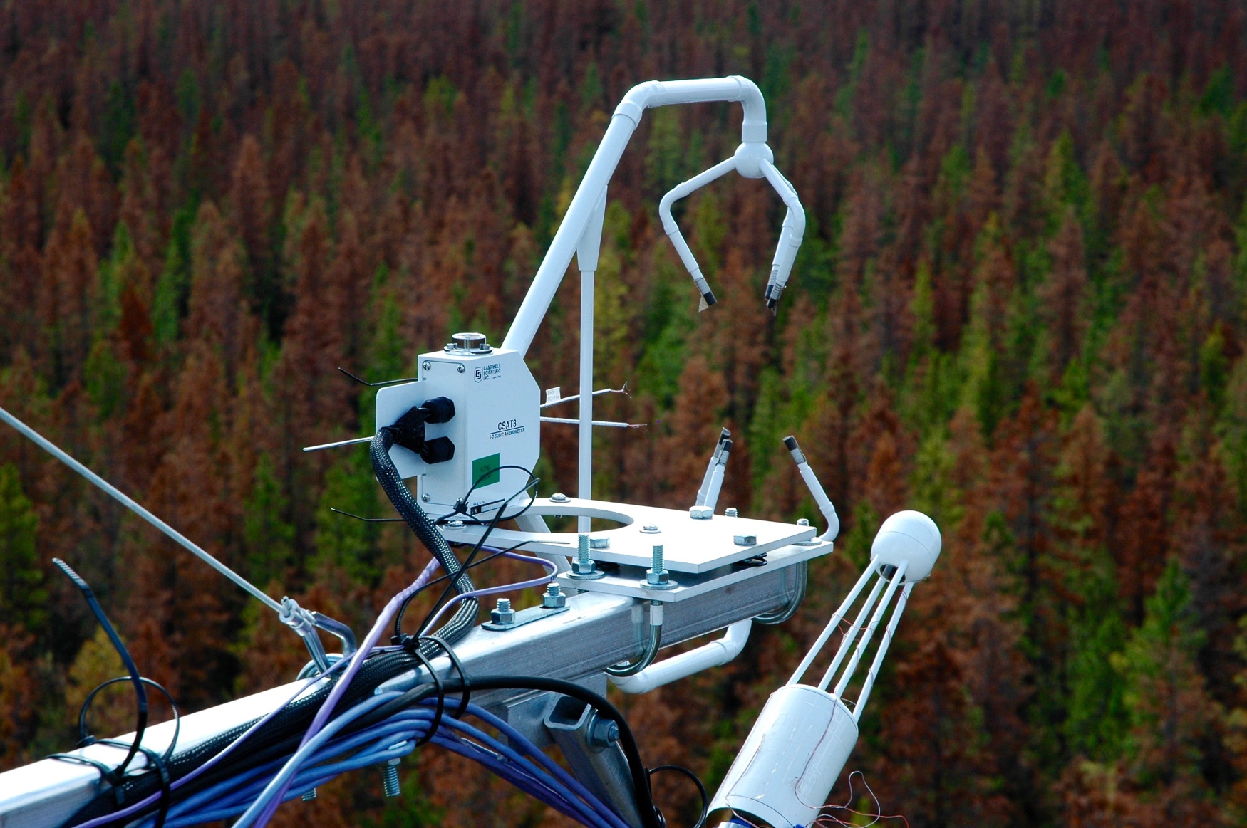
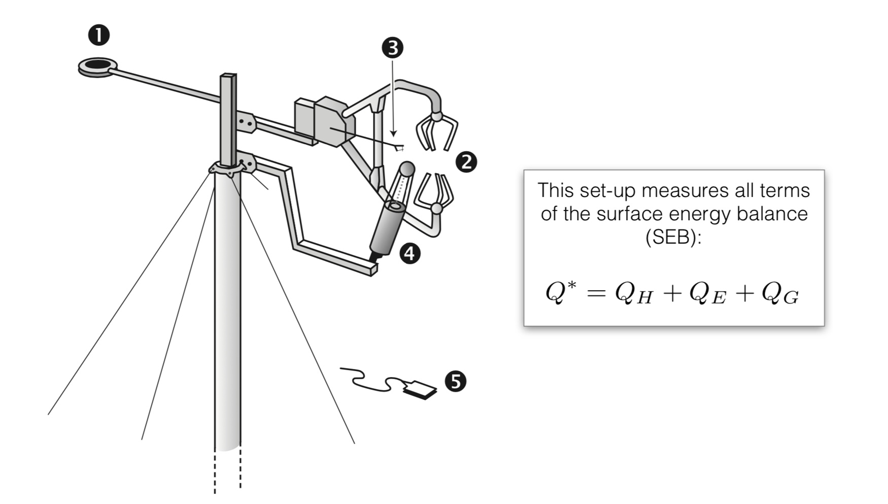
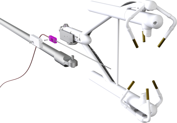
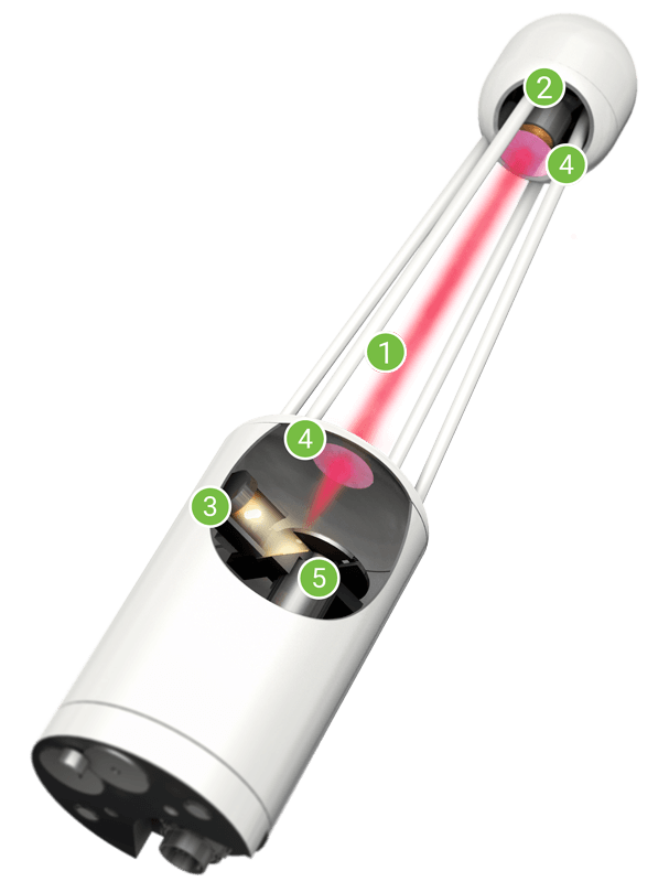
Key Components of an EC System

1. Net all-wave radiometer

Measures total incoming and outdoing radiation (short- and long-wave)

:::

::::

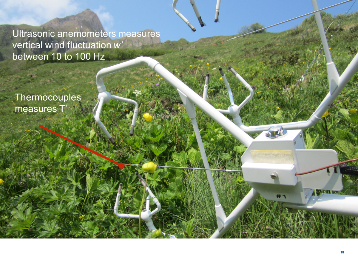
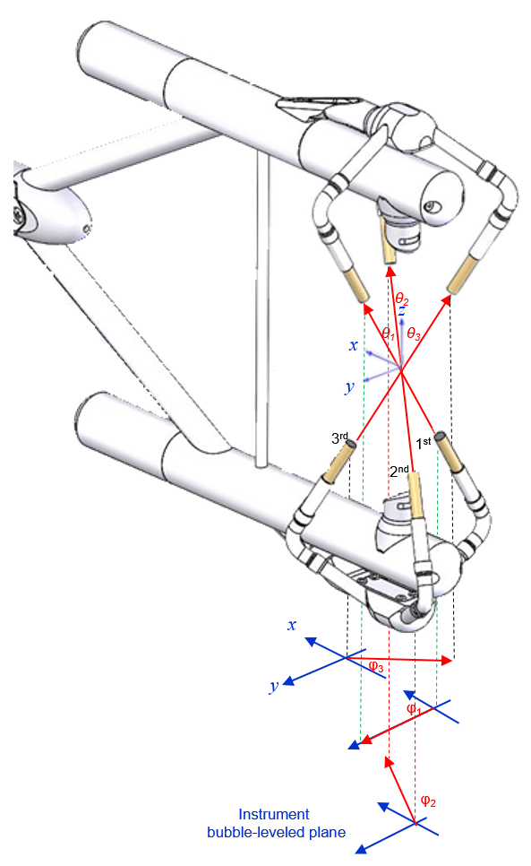
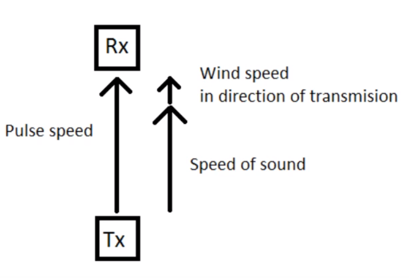
2. 3-D Sonic Anemometer

Travel time of sound pulses between transducers is effected to speed of wind

3. Fine-Wire Thermocouple

Gives fast response, high-precisions temperatures observations.

4. Infrared CO2/H2O gas analyzer

The gas analyzer operates by measuring the absorption of infrared radiation at different wavelengths.

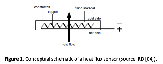
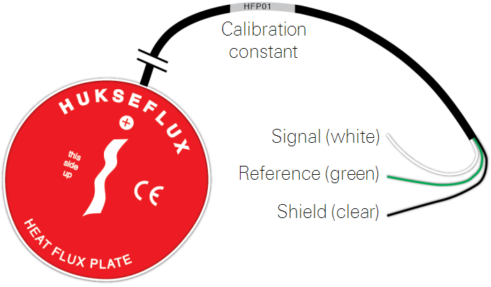
5. Soil heat flux plate

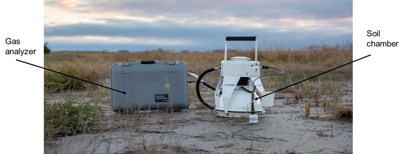
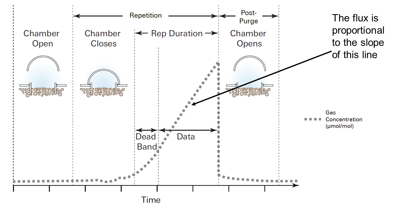
Chamber measurements of GHG fluxes

Chambers placed over the soil can measure soil GHG fluxes at even smaller scales. This requires placing the chamber on top of the soil and measuring the change in gas concentration over time

Chamber measurements of GHG fluxes

Fluxes are calculated based on the change in gas concentration over time (i.e., the slope of the line labeled data).

Take Home Points

• By simultaneously measuring vertical wind and a concentration, we can measure turbulent fluxes using the eddy-covariance technique.
• Eddy-covariance can be used to directly measure the sensible heat flux density using \(H = \rho c_a w’T’\)
• We can track the flux of water vapour and measure the latent heat flux density using \(LE = L_v w’ρv’\)
• To measure traces gas fluxes we use the covariance between the molar density and the vertical wind (w’ρc’)
• Eddy covariance observations can help inform carbon cycle & climate science