Flux-gradient Relations

Learning Objective

• Explain what can we learn from electrical circuits (Ohm’s Law) to describe heat and mass transfer on a land-atmosphere interface.
• Discuss is we can we use the K-Theory introduced for the momentum transfer to relate the gradients of temperature, humidity and trace gas concentrations to fluxes.
• Making the K-Theory useful - Reynold’s analogy (similarity) and aerodynamic approach.

K theory: eddy diffusivities – the ability of eddies to transport mass and energy

Energy balance and turbulence

\[ \color{orange}{R_n} = \color{red}{H} + \color{blue}{LE} + \color{purple}{G} + \color{green}{\Delta S} \tag{1}\]

DeltaQp = net biochemical energy storage in the biomass through photosynthesis minus respiration The common term in the water and energy balance equations is evaporation. To assimilate one mole of CO2, it requires an energy of 469 kJ.

Turbulent exchange

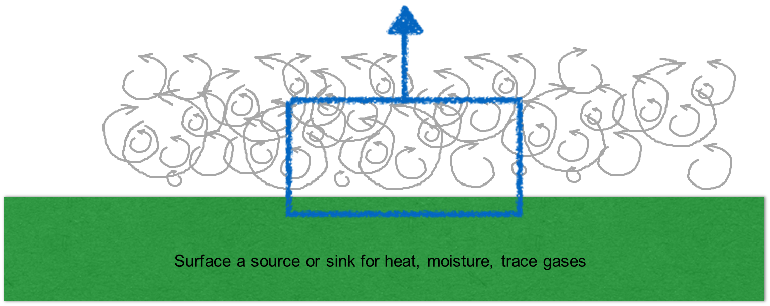
Vertical turbulent flux of sensible heat, latent heat and trace gases

Resistance Approach - Ohm’s Law

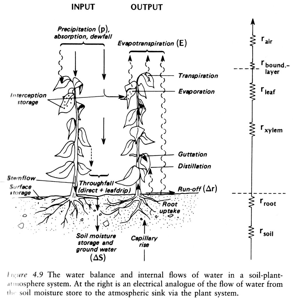
• To describe land-atmosphere exchange of heat, mass and momentum we can identify resistances of different sub-processes, e.g. of plant components (leaf, xylem, root, etc.), soil, whole PBL, etc.
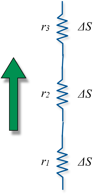
• Resistance relate the flux to a measured difference Δs across part of a system. For a given difference:
• Low resistance - high flux densityHigh resistance - low flux density

Oke (1987)

Inspired by Ohm’s Law

We can define a scalar flux (\(F_c\) in \(m^{-2} s^{-1}\)) in terms of storage (\(\Delta S\) in \(m^{-3}\)) and either resistance (\(r\) in \(s m^{-1}\)) or conductance (\(g\) in \(m s^{-1}\)):

\[ F_c = \frac{\Delta S}{r} \tag{2}\]

\[ F_c = g \Delta S \tag{3}\]

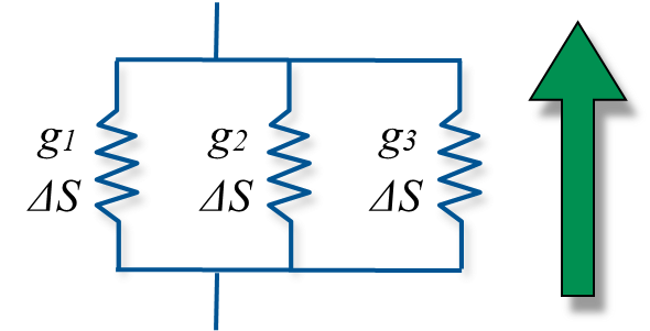
Resistances vs. Conductances

Resistances are additive in series

Conductances are additive in parallel

Resistances at the surface-atmosphere interface

• Several types of resistances / conductances can be conceived of, depending on the transport processes in the layer, e.g.
• \(r_a\) (or \(g_a\)) - aerodynamic resistance (conductance) in the turbulent surface layer. Depends on degree of turbulent activity.
• \(r_b\) (or \(g_b\)) - laminar boundary layer resistance (conductance) in the LBL immediately adjacent to surfaces. Depends on molecular diffusivities and thickness is the key variable.
• \(r_s\) (or \(g_s\)) - stomatal resistance (conductance) of leaf pores. Depends on stomatal aperture (light, T, VPD, \(CO_2\) conc., leaf water potential)
• \(r_c\) (or \(g_c\)) - canopy or surface resistance (conductance). Integrated resistance of complete surface system including \(r_s\) and \(r_b\) of leaves and air in canopy.

aerodynamic resistance (drag): The frictional impedance offered by air to the motion of bodies passing through it.

Aerodynamic resistances

\[ \tau = \rho \frac{\Delta\bar{u}}{r_{aM}} \approx \rho \frac{\bar{u_z}}{r_{aM (0-z)}} \tag{4}\]

• Where \(\tau\) is momentum flux density (in \(N m^{-2}\) aka \(Pa\))
• \(r_{aM}\) is aerodynamic resistance (in \(s m^{-1}\))
• \(\bar{u_z}\) is mean wind speed at z (in \(m s^{-1}\))
• \(\rho\) is density of air (in \(kg m^{-3}\))

\[ H = -C_a \frac{\Delta\bar{\Theta}}{r_{aM}} \tag{5}\]

• Where \(H\) is sensible heat flux density (in \(W m^{-2}\) )
• \(\bar{\Theta}\) is mean potential temperature (in \(K\)) see
• \(C_{a}\) is the heat capacity of air (in \(J m^{-3} K^{-1}\)) see

In the turbulent surface layer (define): typically the bottom 10% where the log wind profile is valid Between SURFACE and measurement height!

Aerodynamic resistances

\[ E = - \frac{\Delta\bar{\rho_v}}{r_{av}} \tag{6}\]

• Where \(E\) is water vapor flux density (in \(kg m^{-2} s^{-1}\))
• \(r_{av}\) is aerodynamic resistance (in \(s m^{-1}\))
• \(\bar{\rho_v}\) is mean partial vapor density of water (in \(kg m^{-3}\))

\[ F_c = - \frac{\Delta\bar{\rho_c}}{r_{ac}} \tag{7}\]

• Where \(F_c\) is trace gas flux density (in \(kg m^{-2} s^{-1}\))
• \(r_{ac}\) is aerodynamic resistance (in \(s m^{-1}\))
• \(\bar{\rho_c}\) is mean partial density of the trace gas (in \(kg m^{-3}\))

In the turbulent surface layer (define): typically the bottom 10% where the log wind profile is valid Between SURFACE and measurement height!

Flux-gradient relationships

• For small-scale turbulence, the flux is down the concentration gradient, i.e
  • momentum flux density is fast \(\rightarrow\) slow
  • sensible heat flux density is ?? \(\rightarrow\) ??
  • water vapor flux density is wet \(\rightarrow\) dry
  • trace gas flux density is high concentration \(\rightarrow\) low concentration

Boussinesq suggested that turbulent transfer could be considered analogous to molecular diffusion - eddies replace molecules:

• Flux density = transfer efficiency \(\times\) gradient of entity

Photo: A. Christen

If we have more momentum at a higher layer (rhoubar) than a lower layer (rhoubar) , a potential gradient in momentum will be established. Momentum will flow from the region of higher momentum to that of lower momentum. So, momentum must be transferred downward. Which are analogous to Fourier’s and Fick’s laws of molecular diffusion of heat and mass.

Sensible Heat Flux Density (iClicker)

Sensible heat flux density is directed from ?? \(\rightarrow\) ??

• A cold \(\rightarrow\) hot
• B hot \(\rightarrow\) cold
• C dry \(\rightarrow\) wet
• D sunny \(\rightarrow\) dark

Photo: A. Christen

If we have more momentum at a higher layer (rhoubar) than a lower layer (rhoubar) , a potential gradient in momentum will be established. Momentum will flow from the region of higher momentum to that of lower momentum. So, momentum must be transferred downward. Which are analogous to Fourier’s and Fick’s laws of molecular diffusion of heat and mass.

K-Theory

If \(K_M\), \(K_H\), \(K_V\) and \(K_C\) are eddy diffusivities (in \(m^2 s{-1}\)).

\[ \tau = \rho K_m \frac{\delta\bar{u}}{\delta z} \]

\[ LE = -K_v \frac{\delta\bar{\rho_v}}{\delta z} \]

\[ H = -C_a K_H \frac{\delta\bar{\Theta}}{\delta z} \]

\[ F_c = -K_c \frac{\delta\bar{\rho_c}}{\delta z} \]

Which are analogous to Fourier’s and Fick’s laws of molecular diffusion of heat and mass. Km analogous to the molecular kinematic viscosity v. Transfer efficiency It should be recognized that the above gradient-transport relations are not the expressions of any sound physical laws in the same sense that their molecular counterparts are. These are not based on any rigorous theory, but only on an intuitive assumption of similarity or analogy between molecular and turbulent transfers. Under ordinary circumstances, one would expect heat to flow from warmer to colder regions, roughly in proportion to the temperature gradient.

K-Theory - limitations

• K’s are extremely variable in time, space and atmospheric conditions (stability).
• Requires instruments capable of measuring small vertical gradients (differences) to high accuracy.
• Also the K-theory does not account for counter-gradient transport.
  • In the atmosphere, sometimes fluxes are counter gradient. Due to a large eddies which (briefly) transport flux regardless of background average (e.g. within plant canopies)

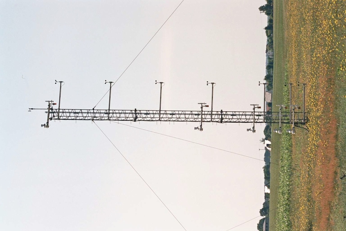
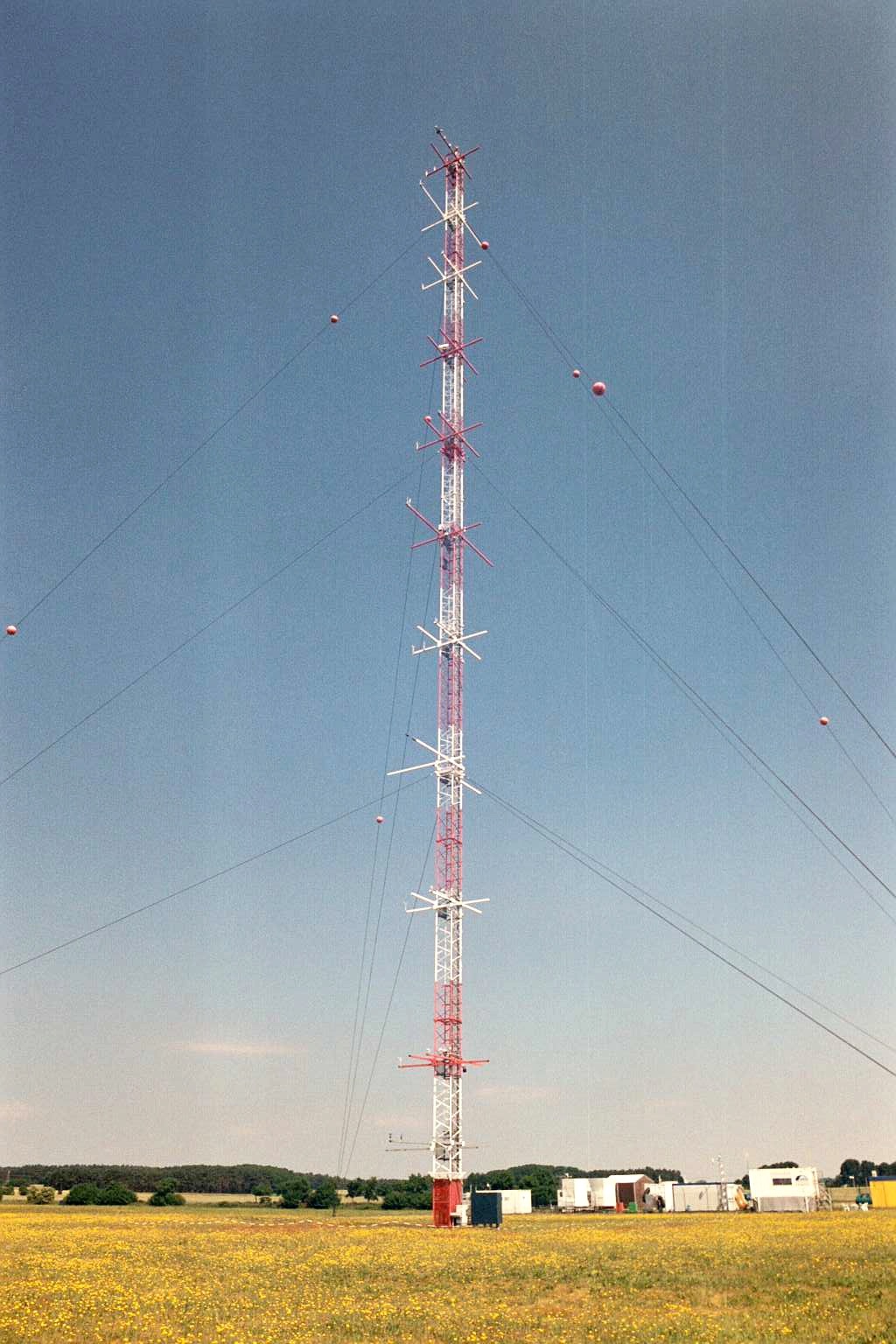
A 100m profile research tower probing theatmospheric surface layer (Falkenberg, DWD, Photo: A. Christen)

eddy diffusivities The observation of a secondary wind maxima suggests counter-gradient transfer since momentum transfer is directed downward and is diminishing with depth, despite the local increase in wind velocity. It also led to a major finding that K theory is wrong, when applied in vegetation. Wilson and Shaw [N R Wilson and Shaw, 1977] applied a second order closure model to assess this phenomenon. It should be recognized that the above gradient-transport relations are not the expressions of any sound physical laws in the same sense that their molecular counterparts are

Reynolds Analogy

Reynolds surmised that in fully turbulent flow (high \(R_e\)) eddies would carry entities with equal ease (similarity principle):

\(K_m = K_H = K_v = K_c\)

• and consequently, over the same layer

\(r_{am} = r_{aH} = r_{av} = r_{ac}\)

• Practically this implies that we must only determine one of the K’s

• Generally held that close to the ground this applies, except that \(K_M\) becomes increasingly dissimilar as instability increases, and then:

\(K_x \propto K_M^2\)

Using K-theory & Reynold’s Analogy to measure fluxes

Assumptions:

• Neutral stability: buoyancy effects are absent.

• Steady state: no marked shifts in the radiation or wind fields during the observation period.
• Constancy of fluxes with height: no vertical divergence or convergence.
• Similarity of all transfer coefficients.

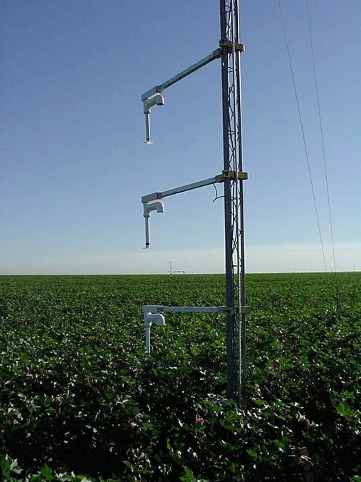
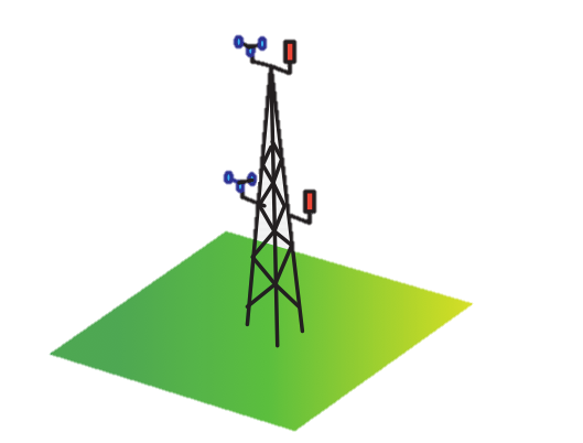
2 x Anemometer & 2 x Thermometer-Hygrometer

In the turbulent surface layer (define): typically the bottom 10% where the log wind profile is valid

Reynolds Analogy

If we assume a similarity, we can take ratios of flux-gradient equations, and eliminate the K’s. If one flux is known (usually \(\tau\) from a measured wind profile), we can obtain other if their gradients are measured, e.g.

\[ \frac{\tau}{H} = \frac{\cancel{\rho}\cancel{K_M}(\Delta\bar{u}/\cancel{\Delta z})}{-\cancel{\rho}c_a\cancel{K_H}(\Delta\bar{\Theta}/\cancel{\Delta z})} = \frac{\Delta \bar{u}}{-c_a \Delta \bar{\Theta}} \tag{8}\]

• where \(C_a = \rho c_a\)

Potential temperature

Aerodynamic Approach

The aerodynamic approach requires the measurement [or prediction in a model] of mean wind u and relevant property (e.g. potential temperature \(\Theta\) absolute humidity \(\rho_v\) ) at same two heights [or layers]. It relies on the similarity of \(K_M\) and \(K_x\).

Assumptions:

• Neutral stability - buoyancy effects are absent.
• Steady state - no marked shifts in the radiation or wind fields during the observation period.
• Constancy of fluxes with height - no vertical divergence or convergence.
• Similarity of all transfer coefficients.

2 x Anemometer & 2 x Thermometer-Hygrometer

In the turbulent surface layer (define): typically the bottom 10% where the log wind profile is valid

Aerodynamic Approach ( 1/3)

From the neutral wind law:

\[ \begin{align} \bar{u_2} =\frac{u*}{k} (ln z_2 - ln z_0) \\ \nonumber \bar{u_1} =\frac{u*}{k} (ln z_1 - ln z_0) \\ \nonumber (\bar{u_2} - \bar{u_1})=\frac{u*}{k} (ln z_2 - ln z_1) \nonumber \end{align} \]

rearranging:

\[ \frac{\Delta \bar{u}}{ln(z_2/z_1)} = u_*/k \tag{9}\]

Aerodynamic Approach ( 2/3)

Since \(\tau \approx \rho u_*^2\); we can redefine:

\[ \tau = \rho k^2 [\Delta\bar{u}/ln(z_2/z_1)]^2 \tag{10}\]

And substitute Equation 10 into Equation 8 and solve \(H\)

Aerodynamic Approach ( 3/3)

For Sensible Heat Flux (\(H\)):

\[ \begin{align} H&=\frac{-\tau c_a \Delta\bar{\Theta}}{\Delta\bar{u}} \\ \nonumber &=\frac{-\rho k^2 \Delta\bar{u}^2c_a \Delta\bar{\Theta}}{\Delta\bar{u}[ln(z_2/z_1)]^2} \\ \nonumber &=\frac{-\rho k^2 \Delta\bar{u} c_a \Delta\bar{\Theta}}{[ln(z_2/z_1)]^2} \end{align} \tag{11}\]

For Latent Heat Flux (\(LE\)):

\[ LE = -\frac{L_v k^2 \Delta\bar{u} \Delta\bar{\rho_v}}{[ln(z_2/z_1)]^2} \]

2 x Anemometer & 2 x Thermometer-Hygrometer

Specific heat of air

Take Home Points

• Resistance allow us to handle the flow of energy and mass though a complex system such as a land-atmosphere interface. Resistances can be formulated in series or in parallel.
• Resistance formulations and flux-gradient relations (using eddy diffusivities, i.e. K’s) can be used to describe sensible, latent heat and trace gas transfer.
• Reynolds analogy assumes that the eddy diffusivities for different scalars are similar, i.e. \(K_M\) = \(K_H\) = \(K_E\) = \(K_C\)
• This allows us to overcome the severe restrictions of using K-theory - as in the aerodynamic approach the K’s cancel out.