Velocity Profile Laws

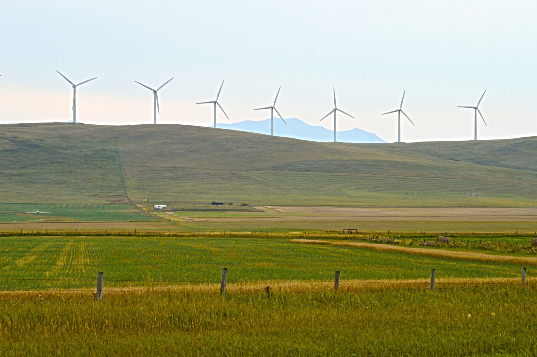
General characteristics of how wind speed varies with height

For any given weather condition, there is a theoretical equilibrium wind speed, called the geostrophic wind \(G\), that can be calculated for frictionless conditions. However, steady-state winds in the ABL are usually slower than geostrophic (i.e., subgeostrophic) because of frictional and turbulent drag of the air against the surface.

Today’s learning objectives

• Describe how the mean velocity profile is linked to the momentum flux.
• Understand the ‘famous’ logarithmic wind profile equation.

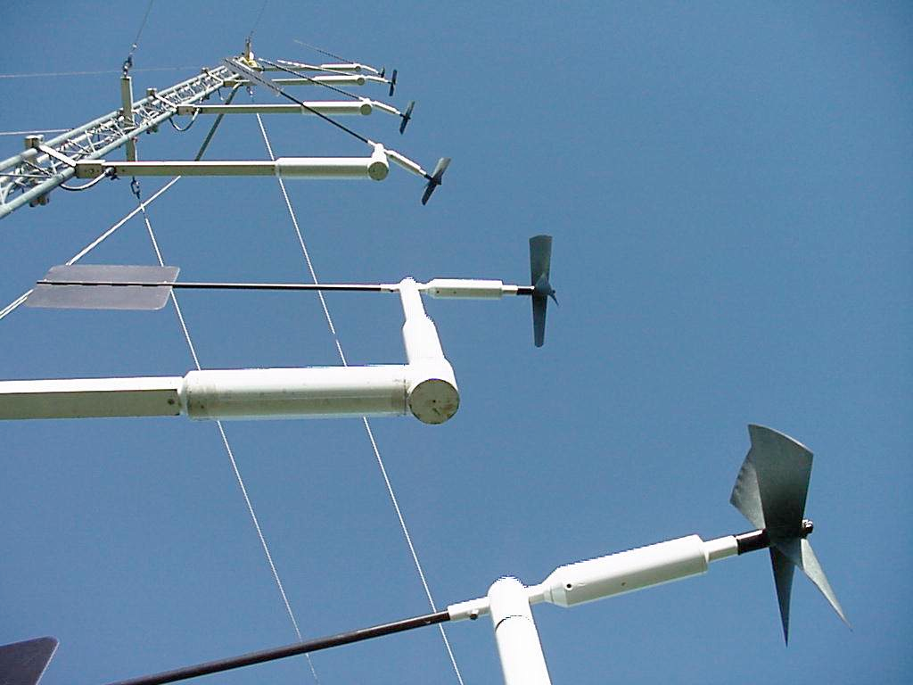
The vertical profile of horizontal wind

Series of anemometers at different heights z over an extensive flat

This is the vertical profile of mean horizontal wind ū and shows that the wind gradient (or ‘wind shear’) decreases as z increases.

The drag slows motion close to the ground and gives rise to a sharp decrease of mean horizontal wind speed (u) as the surface is approached. The force exerted on the surface by the air being dragged over it is called the surface shearing stress (tau ) and is expressed as a pressure (Pa, force per unit surface area). The surface layer of frictional influence generates this shearing force and transmits it downwards as a flux of momentum.

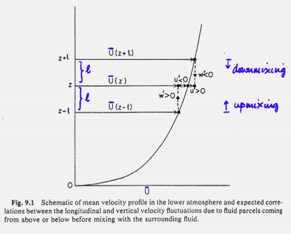
Mixing Length

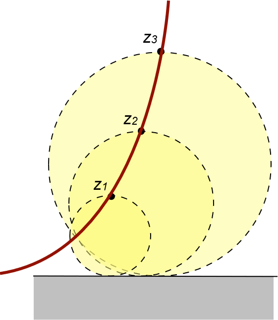
The characteristic height for mixing to occur is the mixing length \(l\) and is likely related to the mean size of eddies.

Assume an eddy at level (\(z+l\)) with mean velocity \(\bar{u}_{(z+l)}\) moves down to \(z\) where mean velocity \(\bar{u}_{(z)}\) is less, by \(u^{\prime}\):

\[ u^{\prime} = \bar{u}_{(z+l)}-\bar{u}_{(z)} \]

so: \[ u^{\prime} = l\small\frac{\delta u}{\delta z} \qquad(1)\]

• i.e. extra velocity = increment in height x rate of change of velocity with height.

Mixing length is related to mean size of eddies. The characteristic height difference for mixing to occur is the mixing length l

The mixing length approach

If turbulence is assumed to be isotropic (\(u^{\prime} \approx w^{\prime}\)), i.e., eddies are symmetric:

• \(\tau = -\rho u^{\prime}w^{\prime} \approx \rho u_*^2\) (see previous lecture) it follows \(u^{\prime} \approx w^{\prime} \approx u_*\) and we can define \(u_*\) in terms of the mixing lenght:

\[ \small\frac{\delta \bar{u}}{\delta z} = \small\frac{u_*}{l} \]

• i.e. the wind gradient is inversely related to the size of the eddies. As we approach the ground the spectrum of eddy sizes is restricted by the physical barrier.

If we take this mixing length approach, we can re-write this in terms of friction velocity: is a form by which a shear stress may be re-written in units of velocity

mixing length l and is likely related to the mean size of eddies.

The mixing length approach

If turbulence is assumed to be isotropic (eddies are symmetric) \(u^{\prime} \approx w^{\prime}\) and \(\tau = -\rho u^{\prime}w^{\prime}\) and \(\tau = \rho u_*^2\) (see previous lecture) it follows \(u^{\prime} \approx w^{\prime} \approx u_*\) and we can write:

\[ \small\frac{\delta \bar{u}}{\delta z} = \small\frac{u_*}{l} \qquad(2)\]

• i.e. the wind gradient is inversely related to the size of the eddies. As we approach the ground the spectrum of eddy sizes is restricted by the physical barrier.

mixing length l and is likely related to the mean size of eddies. WRITE ON BOARD

Shear Velocity, also called friction velocity, is a form by which a shear stress may be re-written in units of velocity. It is useful as a method in fluid mechanics to compare true velocities, such as the velocity of a flow in a stream, to a velocity that relates shear between layers of flow. Shear velocity is used to describe shear-related motion in moving fluids. It is used to describe: Diffusion and dispersion of particles, tracers, and contaminants in fluid flows The velocity profile near the boundary of a flow (see Law of the wall) Transport of sediment in a channel

The vertical profile of horizontal wind

The form of the vertical profile of horizontal wind is found to be:

\[ \small\frac{\delta \bar{u}}{\delta z} = a(z)^{-b} \qquad(3)\]

• The form says \(\bar{u}\) is proportional to the logarithm of \(z\)
  • Extensively verified in the field and laboratory.

Parameter a

von Kármán’s constant

So if the eddy size is proportional to the distance to the ground, let’s set \(l=k(z)^b\), in neutral stability: \(b = 1 \rightarrow l=kz\)

• and therefore, substitution of \(l\) into Equation 2 gives

\[ \frac{\delta \bar{u}}{\delta z} = \frac{u_*}{k}(z)^{-b} = \frac{u_*}{kz} \qquad(4)\]

• i.e. in Equation 3; \(a=u_*/k\)

The constant \(k\) is von Kármán’s constant (\(\approx\) 0.41)

The logarithmic wind law

Integration of Equation 4 requires knowledge of the exact height where is \(\bar{u}\) zero (integration constant). In practice this depends on the roughness of the ground so we set a roughness length (\(z_0\), units m) and restrict the equation to \(z > z_0\).

\[ \bar{u_z}=\frac{u_*}{k}ln(\frac{z}{z_0}) \qquad(5)\]

• This is the log wind law for neutral conditions. The general form for measurements in two levels:

\[ \bar{u_2}-\bar{u_1}=\small\frac{u_*}{k}ln(\small\frac{z_2}{z_1}) \qquad(6)\]

neutral conditions where buoyancy is unimportant. Such conditions are found with cloudy skies and strong winds, and in the lowest 1 to 2 m of the atmosphere.

Linear-Log Plot of Neutral Wind Profile

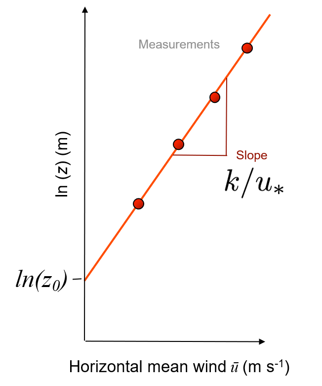
In neutral conditions, the slope of wind speed with \(ln(z)\) is exactly linear and both, \(u_*\) and \(z_0\) can be determined from analysis of wind data from several levels.

• The y-intercept on a log-linear plot will give us \(z_0\)
• The slope on a log-linear plot will give us \(k/u_*\)

neutral conditions where buoyancy is unimportant. Such conditions are found with cloudy skies and strong winds, and in the lowest 1 to 2 m of the atmosphere.

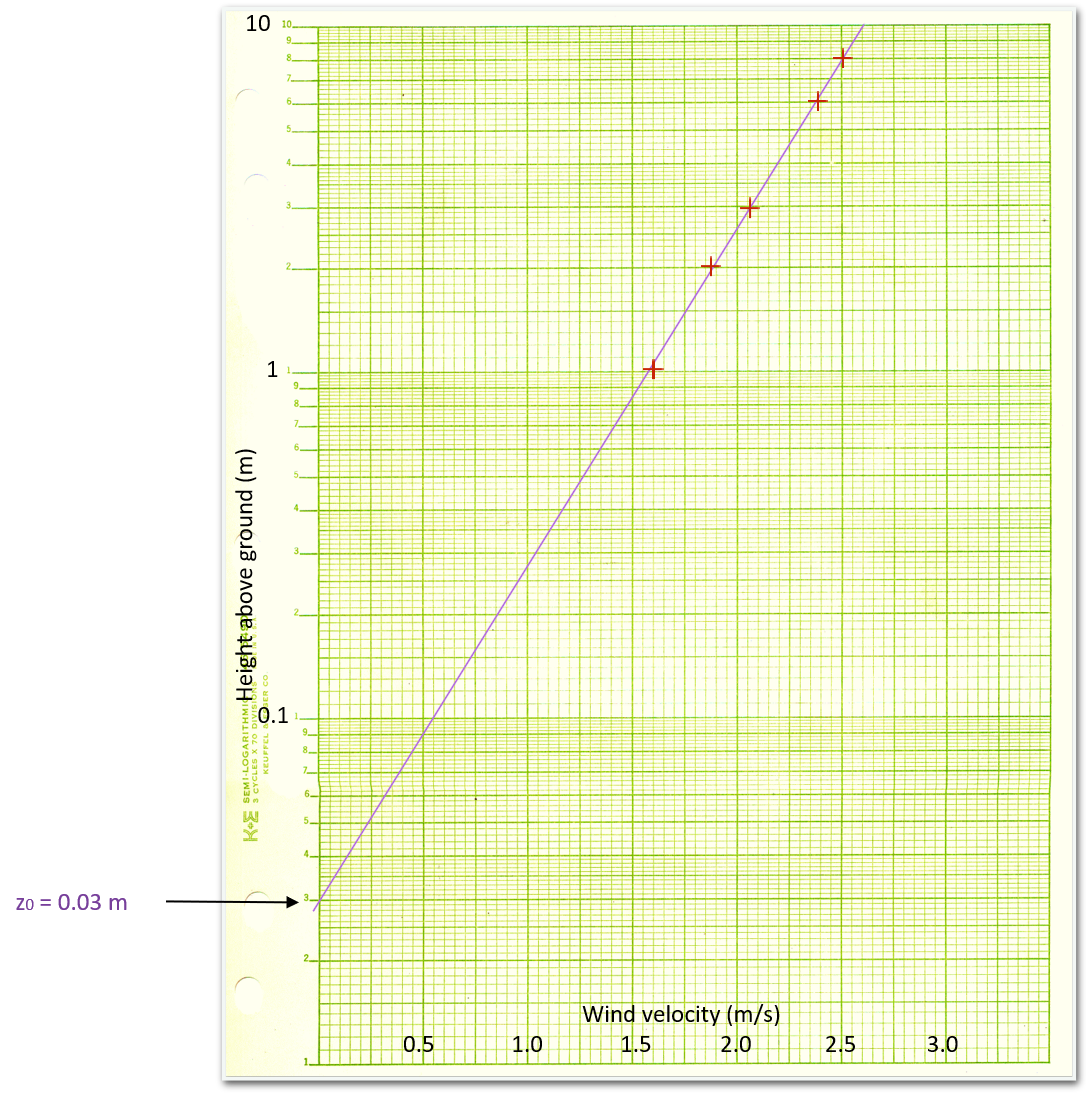
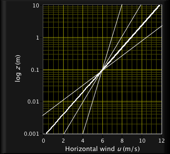
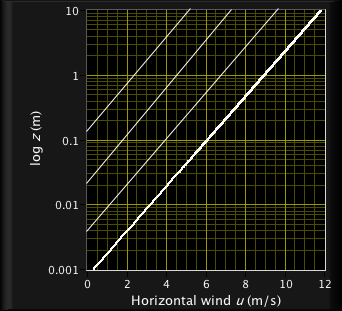
Semi-log paper

On this paper, you can directly enter wind velocity on the x-axis (linear scale) and height on the y-axis (logarithmic scale).

First label your own axes (orders of magnitude on y-axis) to fit data optimally on paper. Then enter data points.

You can fit a line (e.g. by hand using a ruler). The intercept with the y-axis gives you an estimate of z0.

Make Your Own Log-Plot

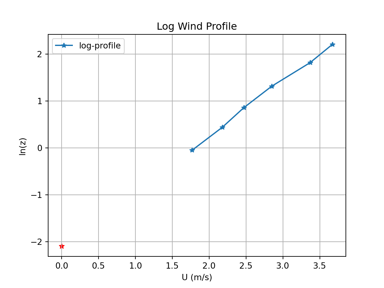
import pandas as pd
import numpy as np

# Load a wind profile
profile = pd.read_csv('Data/Profile.csv')
# Calculate ln(z)
profile['lnz']=np.log(profile['z (m)'])
# Find the intercept of a linear fit
m,b=np.polyfit(profile['u (m/s)'],profile['lnz'],1)

print(f'm = {m}; b = {b}')

m = 1.1751196328367708; b = -2.0986472898421247

import matplotlib.pyplot as plt
# Plot the results
fit,ax=plt.subplots()
profile.plot(x='u (m/s)',y='lnz',ax=ax,marker='*',label='log-profile')
ax.scatter(0,b,marker='*',color='r',label='intercept')
ax.grid()
ax.set_title('Log Wind Profile')
ax.set_ylabel('ln(z)')
ax.set_xlabel('U (m/s)')

Log-Profile (iClicker)

import pandas as pd
import numpy as np

# Load a wind profile
profile = pd.read_csv('Data/Profile.csv')
# Calculate ln(z)
profile['lnz']=np.log(profile['z (m)'])
# Find the intercept of a linear fit
m,b=np.polyfit(profile['u (m/s)'],profile['lnz'],1)

print(f'slope (m) = {m}; intercept (b) = {b}')

slope (m) = 1.1751196328367708; intercept (b) = -2.0986472898421247

From this, what would be the value of \(z_0\) in meters?

• A \(z_0 = b\)
• B \(z_0 = ln(b)\)
• C \(z_0 = e^{b}\)
• D \(z_0 = e^{m}\)
• E \(z_0 = ln{m}\)

Log-Profile (iClicker)

import pandas as pd
import numpy as np

# Load a wind profile
profile = pd.read_csv('Data/Profile.csv')
# Calculate ln(z)
profile['lnz']=np.log(profile['z (m)'])
# Find the intercept of a linear fit
m,b=np.polyfit(profile['u (m/s)'],profile['lnz'],1)

print(f'slope (m) = {m}; intercept (b) = {b}')

slope (m) = 1.1751196328367708; intercept (b) = -2.0986472898421247

From this, what would be the value of \(u_*\) in meters per second?

• A \(u_* = m\)
• B \(u_* = 0.41 \times m\)
• C \(u_* = 0.41 \times b\)
• D \(u_* = b\)
• E \(u_* = b / 0.41\)

Relation between z0 and mean wind speed

See an interactive visualization here

Same reference velocity $u_{ref} but different \(z_0\) and shear stress

Same shear stress but different roughness

As shear stress decreases our slope increases (and z0 decreases too) Shear = slope = u* Rougher surface we have, the lower the windspeed at a given height

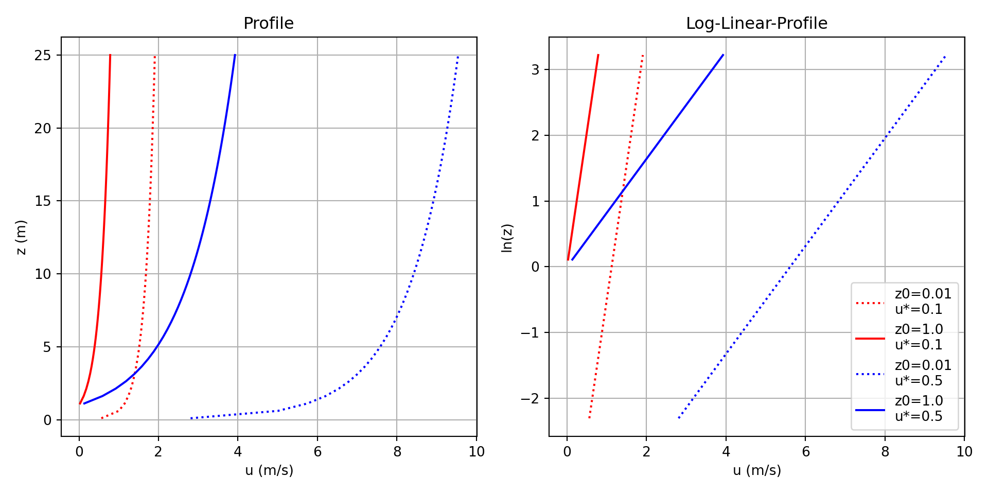
Try yourself

import numpy as np
import matplotlib.pyplot as plt

k = 0.41
# short grass (0.01), trees (1.0)
z0_list = [0.01,1.0] 
# weak winds (0.1), moderately strong winds (0.5)
u_star_list = [0.1,0.5]
# define a height profile
z = np.linspace(0.1,25)
# define a plot and loop through scenarios
fig,ax=plt.subplots(1,2)
for u_star,c in zip(u_star_list,['r','b']):
    for z0,l in zip(z0_list,[':','-']):
        u_bar_z = u_star/k*np.log(z/z0)
        u_bar_z[u_bar_z<0]=np.nan
        ax[0].plot(u_bar_z,z,color=c,linestyle=l)
        ax[1].plot(u_bar_z,np.log(z),label=f'z0={z0}\nu*={u_star}',color=c,linestyle=l)
# format the graph
ax[1].legend()
ax[0].set_ylabel('z (m)')
ax[0].set_title('Profile')
ax[1].set_ylabel('ln(z)')
ax[1].set_title('Log-Linear-Profile')
for a in ax:
    a.set_xlabel('u (m/s)')
    a.grid()
plt.tight_layout()

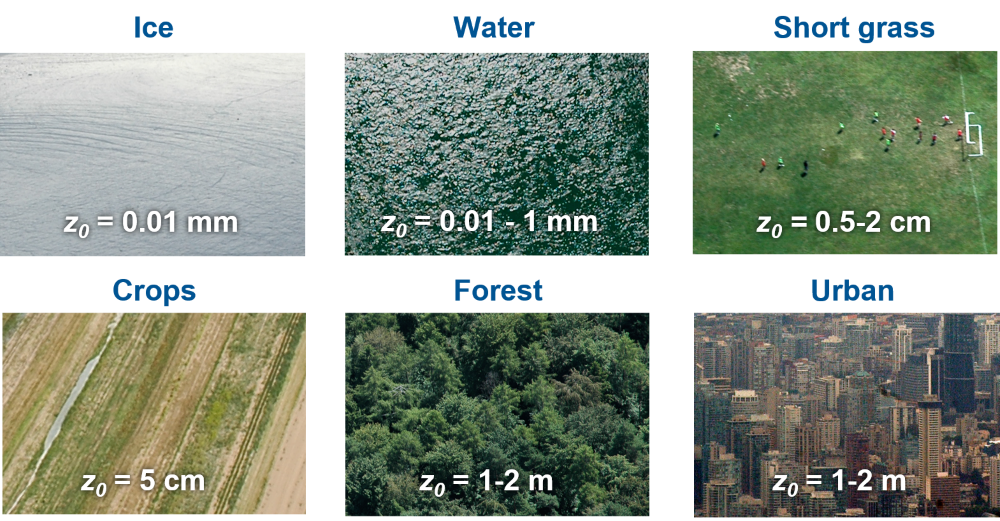
Roughness length \(z_0\) - examples

Estimating the roughness length z0

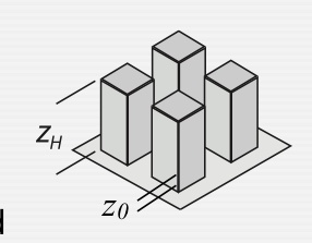
If observations are not available, a first order estimate of z0 can be obtained from a geometric analysis of the surface roughness elements.

• A traditional rule-of-thumb gives: \(z_0 = 0.1\)

Wind profiles over different surfaces

T.R. Oke (1987): ‘Boundary Layer Climates’ 2nd Edition.

Geostrophic The depth of this layer increases with increasing roughness. Therefore the vertical gradient of mean wind speed (du/dz) is greatest over smooth terrain, and least over rough surfaces. Rougher surface we have, the lower the windspeed at a given height

Tall roughness

Over tall roughness elements (such as tall vegetation, orchards, forests) a dead zone in amongst the elements exists.

• This causes the form of the wind profile to diverge from observations, wind seems to go to zero at z >> z0.

Zero-plane displacement \(z_d\)

• We introduce an effective height of mean drag, the zero-plane displacement \(z_d\):

\[ \bar{u_z}=\small\frac{u_*}{k}ln(\frac{z-z_d}{z_0}) \qquad(7)\]

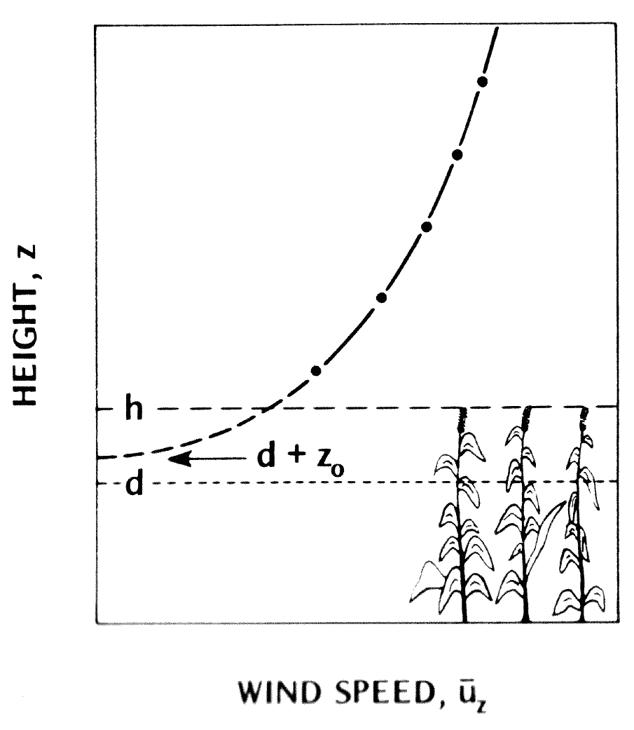
• Over tall roughness elements the straight line plot of ū vs. ln(z) breaks down - so we need to introduce an effective height of mean drag - zero plane displacement \(z_d\).

T.R. Oke (1987): ‘Boundary Layer Climates’ 2nd Edition.

roughness length

Estimating \(z_d\)

• It is possible to determine zd from analysis of wind observations:

  • Iteration using trial values to find \(z_d\) which straightens plot \(\bar{u}\) vs. \(ln(z- z_d)\) under neutral conditions.

• A rule-of-thumb says: \(z_d = 2/3 z_h\), but it omits density consideration.

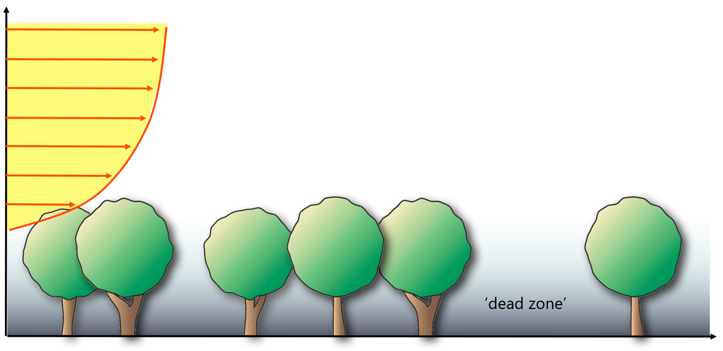
  • \(\bar{u}_z\) should reach zero at the height \(z_d+z_0\).

• However, this is not observed in vegetation canopies.

  • We observe wind speed > 0 even below \(z_d+z_0\).

roughness length

The vertical profile of horizontal wind

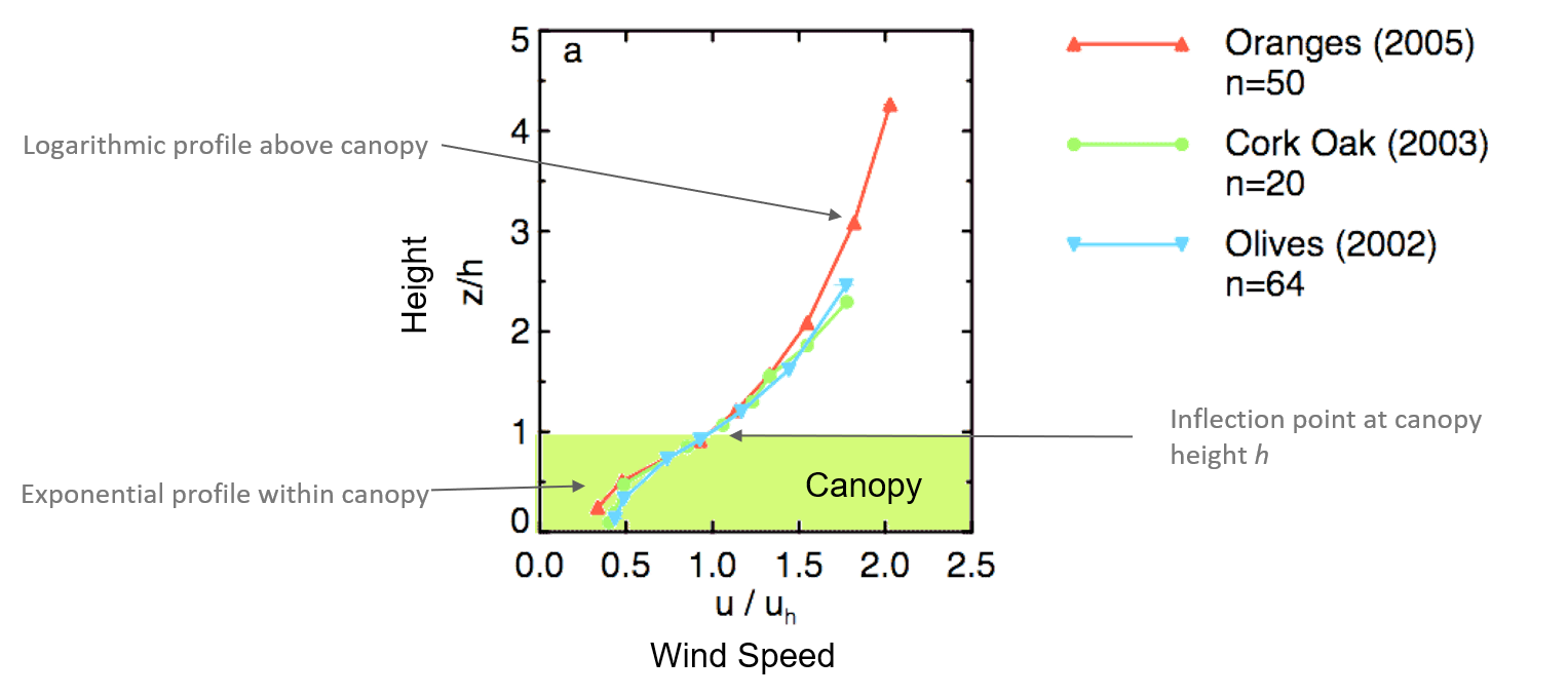
In most canopies (forests, orchards, crops) we find the logarithmic wind profile well above the mean canopy height h, and an exponential profile within the canopy.

The Exponential Wind Profile

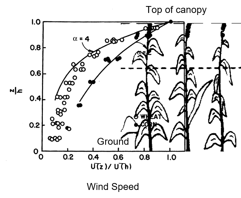
The mean wind profile inside homogeneous canopies can be approximated as exponential function (z < h):

\[ \bar{u}_z=\bar{u}_h e^{\alpha(z/h-1)} \qquad(8)\]

\(\alpha\) is an empirical constant, the canopy’s wind extinction coefficient.

Table 1: Alpha values for different canopies

Wind extinction coefficients	α
Wheat	4.0
Corn	2.0
Sunflower	1.3
Spruce	2.4

S. P. Arya (1998): ‘Introduction to Micrmeteorology’

Take home points

• The wind profile in the surface layer follows the logarithmic law.
• The integration constant of the log-law is the roughness length z0, which depends on the surface’s roughness.
• Over tall roughness elements the straight line plot of ū vs. ln(z) breaks down - so we need to introduce an effective height of mean drag - zero plane displacement zd.