Turbulence Statistics
Using statistics to simplify our understanding of turbulence
Learning Objectives
Describe how we can separate turbulent from mean kinetic energy.
Explain how we can quantify turbulence and its properties.
Statistical Approach
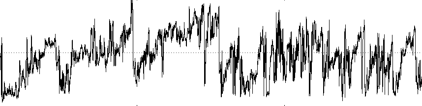
Single motions in a turbulent flow are chaotic and unpredictable. Luckily, they are seldom important,
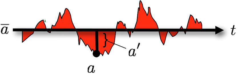
Reynolds Decomposition
Turbulent properties appear chaotic, but can be analyzed by deconstructing them into two parts:
The time mean (e.g., \(\bar{a}\) )
The instantaneous deviation from the mean (e.g., \(a^{\prime}\) )
\[
a(t) = \bar{a} + a^{\prime}(t)
\qquad(1)\]
where:
\[
\bar{a} = \small\frac{1}{N}\sum_{i=0}^{N-1}a(t_i)
\qquad(2)\]
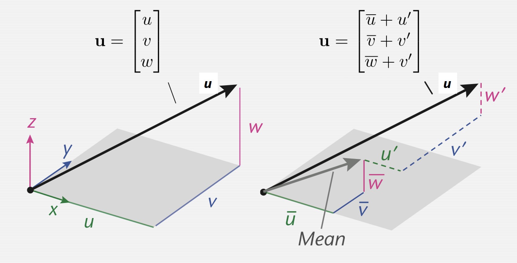
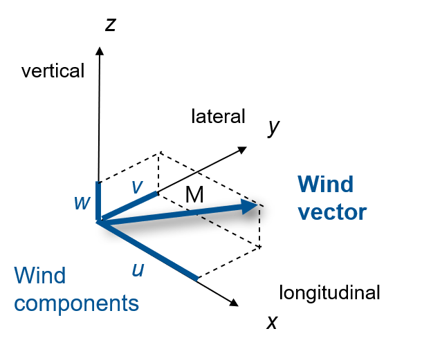
Wind vector has u, v, & w components
A vector is a mathematical object that has a size, called the magnitude, and a direction.
Reynolds Decomposition: Covariance
By definition the average of all fluctuations must vanish.
\[
\begin{align}
\bar{a^{\prime}} = 0 \nonumber \\
\bar{a }\times \bar{b^{\prime}} = 0 \nonumber \\
\overline{a \times b} =\overline{(\bar{a}+a^{\prime})\times(\bar{b}+b^{\prime})} = \bar{a}\times\bar{b} + \overline{a^{\prime}\times b^{\prime}}
\end{align}
\qquad(3)\]
We conclude: A covariance is not necessarily vanishing. Covariances are often very important terms in turbulence.
The covariance indicates the amount of common variation between two variables. It is positive where both variables increase or decrease together. Covariance is negative for opposite variation, such as when one variable increases while the other decreases. Covariance is zero if one variable is unrelated to the variation of the other. “eddy flux” is computed as a covariance between instantaneous deviation in vertical wind speed (w’) from the mean value (w-overbar) and instantaneous deviation in gas concentration, mixing ratio (s’), from its mean value (s-overbar), multiplied by mean air density (ρa). Several mathematical operations and assumptions, including Reynolds decomposition, are involved in getting from physically complete equations of the turbulent flow to practical equations for computing “eddy flux”, as shown below.
Integral Statistics
Also the variance of a in a turbulent time series is not zero. It is defined by:
\[
\overline{a^{\prime2}} = \frac{1}{N}\sum_{i=0}^{N-1}a^{\prime2}(t_i)
\qquad(4)\]
The standard deviation (square root of variance) is in the same units as a:
\[
\sigma_a=\sqrt{\overline{a^{\prime2}}}
\qquad(5)\]
The covariance indicates the amount of common variation between two variables. Variance: Informally, it measures how far a set of (random) numbers are spread out from their average value.
Integral statistics
Turbulence intensities are the dimensionless ratio between the standard deviation and the length of the mean wind vector M.
\[
\begin{align}
I_u = \small\frac{\sigma_u}{M} \nonumber \\
I_v = \small\frac{\sigma_v}{M} \nonumber \\
I_w = \small\frac{\sigma_w}{M} \nonumber \\
M = \sqrt{\bar{u^2} + \bar{v^2} + \bar{w^2}}
\end{align}
\qquad(6)\]
Turbulent Kinetic Energy
Following the definition of kinetic energy (\(E=\frac{1}{2}mv^2\) ) we can define a mean kinetic energy (MKE) per unit mass \(m\) of the flow, namely
\[
\frac{MKE}{m}=\frac{1}{2}(\overline{u^2}+\overline{v^2}+\overline{w^2})
\qquad(7)\]
Similarly, the kinetic energy of the instantaneous deviations per unit mass (e) is:
\[
e=\frac{1}{2}(u^{\prime2}+v^{\prime2}+w^{\prime2}) \nonumber
\]
The average e is called mean turbulent kinetic energy (TKE):
\[
TKE = \overline{e}=\frac{1}{2}(\overline{u{\prime2}}+\overline{v{\prime2}}+\overline{w{\prime2}})
\qquad(8)\]
The TKE budget
TKE in the boundary layer (iClicker)
TKE increases with _______ wind speed.
A increasing
B decreasing
TKE in the boundary layer (iClicker)
TKE is greater over _______ than ________ surfaces.
A rough / smooth
B smooth / rough
TKE in the boundary layer (iClicker)
TKE is greatest in __________ atmosphere, least in ________ atmosphere.
A stable / unstable
B unstable / stable
Probability Densities
A probability density function (PDF) describes the probability of occurrence of a particular value of any parameter.
It is useful to look at the probability density functions of turbulent fluctuations (\(u^{\prime}\) ,\(v^{\prime}\) ,\(w^{\prime}\) ,\(T^{\prime}\) ,\(\rho^{\prime}\) ,etc.).
A histogram is a discrete representation of a probability density.
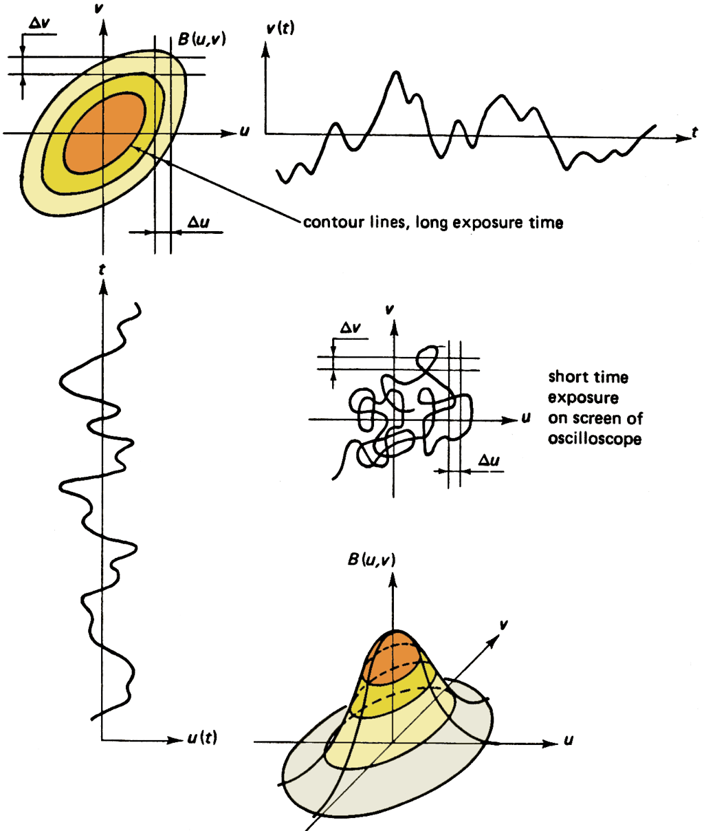
Joint Probability Density
A \(\geq 2D\) probability density of co-occurrence variables is called joint probability density.
This can be very informative, e.g.,:
Say \(w^{\prime}\) and \(\rho_{H_2O}^{\prime}\) are correlated, this gives us information about H2 O transport toward/away from the surface
A joint probability is a statistical measure that calculates the likelihood of two events occurring together and at the same point in time. Joint probability is the probability of event Y occurring at the same time event X occurs. Useful for metrics such as covariance of correlation coefficients Covariance = related to the area under your PDF
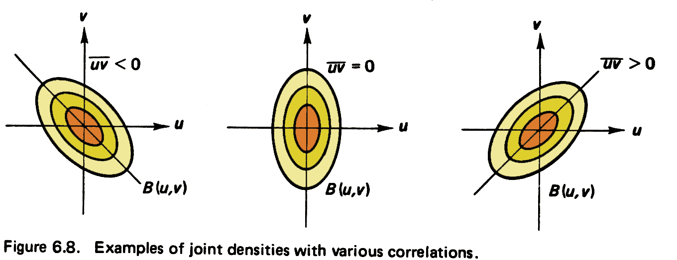
Joint probability density - examples
H. Tennekes and J. L. Lumley (1972): A first course in turbulence. Massachusetts Institute of Technology.
Joint probability density B(u,v)
Correlation coefficient
The correlation coefficient \(r\) describes covariance relative to variability:
e.g., for \(u\) and \(w\) , it would be: \(r_{uw} = \small\frac{\overline{u^{\prime}w^{\prime}}}{\sigma_u \sigma_w}\)
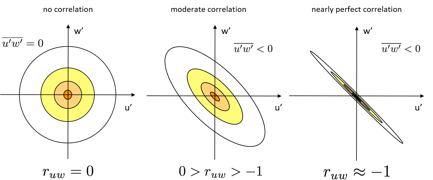
Correlation coefficient is defined as the covariance normalized by the standard deviations for the two variables. Normalizing means -1=> r +< 1. A correlations coefficient of 1 indicates a perfect correlation (both variables increase or decrease together proportionally), -1 means a perfect opposite correlation, and 0 indicates no correlation. Joint probability density. Note the asymmetric PDF –By inspection, note that the larger probabilities occur as X and Y move in opposite directions. This indicates a negative covariance. All values of ruw are well negatively correlated (average -0.3) because wind increases with height In the ABL, many turbulent variables are correlated. E.g. in unstable conditions, parcels of warm air rise while other cool parcels sink in convective circulation (e.g. w’theta’ = postive) The closer the correlation is to 1 or −1, the closer the joint distribution of (x,y) pairs hugs a straight line, with positive or negative slope.
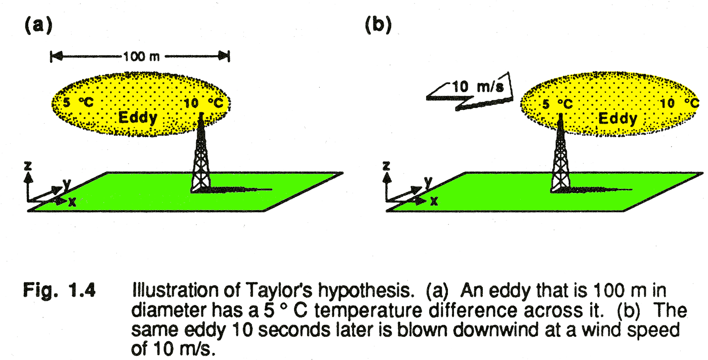
Taylor’s Hypothesis - translating from time to space
\[
\frac{\delta T}{\delta t} = -u \frac{\delta T}{\delta x}
\]
:::
::::
We would like to be able to take snapshots of the eddies in three dimensions and measure all their sizes each instant. Unfortunately, we do not have a good way to do this. Instead, we can simply measure the fluctuations of a variable such as wind speed, specific humidity, or temperature with a sensor at one location for a period of time. In this way, we watch the eddies drift by the sensor. But the eddies could be changing size and shape as they drift by the sensor. Let’s put this physical concept in the context of the total derivative.
Take a variable like temperature, T. We know that the change in T with time at any location (such as where a sensor might be placed) is the sum of the total derivative and the temperature advection: The temperature advection is the change in temperature at the sensor due to the advection of warmer or colder air past the sensor. The total derivative is the change in temperature of an air parcel moving past the sensor. Such a temperature change may be caused by any number of processes, such as the absorption or emission of radiation, condensation or evaporation (latent heating or cooling), or compression and expansion. Taylor’s hypothesis says that we can assume that the turbulent eddies (which we can think of as large air parcels) are frozen as they advect past the sensor and thus the change in temperature within each eddy is negligible: The temperature advection is the change in temperature at the sensor due to the advection of warmer or colder air past the sensor. The total derivative is the change in temperature of an air parcel moving past the sensor. Such a temperature change may be caused by any number of processes, such as the absorption or emission of radiation, condensation or evaporation (latent heating or cooling), or compression and expansion. Taylor’s hypothesis says that we can assume that the turbulent eddies (which we can think of as large air parcels) are frozen as they advect past the sensor and thus the change in temperature within each eddy is negligible:
Local temperature gradients, which might be present from one side of an eddy to another, are advected across the sensor by the mean wind without the eddy changing.
Taylor’s Hypothesis: Frozen turbulence If turbulence is frozen as it moves (or advects) past a sensor, then the characteristics of the turbulence as a function of time might be translated to their measurements in space (i.e., estimate size of eddies from time rate of fluctuations)
https://www.e-education.psu.edu/meteo300/node/737
Take home points
Turbulent flow can be described using the continuum assumption (parcels rather than molecules).
Reynolds decomposition allows to separate the mean from the turbulent part of a time series.
We are rarely interested in the instantaneous values of the turbulent part - but only in the integral effects.
We can use probability distributions to predict exchange efficiency and mixing in a turbulent flow.