Laminar and Turbulent Flow

The Midterm

The mid-term exam is Wednesday March 13th.

• The midterm will be completed asynchronously over canvas. We will not meet in-person on Wednesday the 13th. You can use this time to complete your exam on canvas instead.
• The exam will not be timed. It is not intended to take longer that a normal lecture period (80 minutes), but I want you to have more time if you need it.
  • The exam will be open for 24 hours and may be completed only once.
    • 8 AM Wednesday March 13th to 8 AM Thursday March 24th
    • Late submissions will not be accepted. If you experience extenuating circumstances, contact me before the exam period closes

The Midterm

It will include topics covered through the end of this lecture. Any topics covered in lecture, assignments, or study questions are fair game.

• A collection of multiple choice, fill in the blanks, matching etc. (~65%)
  • May require some simple calculations
  • Will be marked automatically and grades will be posted shortly after the exam closes
• Short answer questions (~35%)
  • May require some simple calculations
  • Will be marked by myself/your TA and posted about a week after the exam closes

Study Questions

Study question sets 1-5 should be submitted before completing the mid-term.

• These account for approximately 2.8% of your final grade and are only marked for completeness.

• As long as you give an answer for each question (right or wrong) you’ll get full credit.

Mid-term (iClicker)

When and where will the midterm be held?

• A: Wednesday March 13th on Canvas
• B: Wednesday March 6th in Person

Mid-term (iClicker)

How long should the mid-term take?

• A: All day! Don’t make any other plans!
• B: About 80 minutes, but you’ll have extra time if needed :)

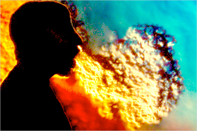
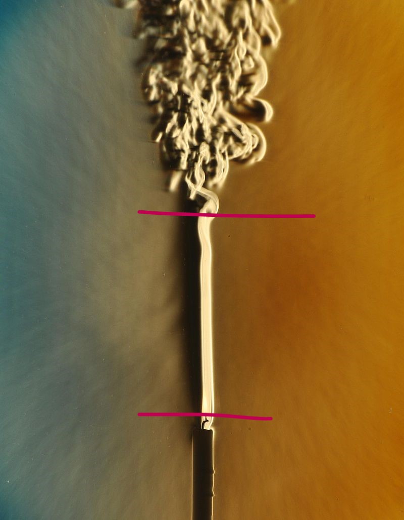
Color schlieren image of a coughing person (Garry Settles, University of Pennsylvania)

Today’s learning objectives

• Define turbulence, and how a turbulent flow differs from a laminar (non-turbulent) one.
• Give examples where flow in the atmosphere is purely laminar.
• Describe how we can describe mass and heat exchange in a laminar flow.

Mechanisms of Energy Transfer

Radiation: electromagnetic waves

Conduction: molecular motion

Convection: mass movement in a fluid

Radiative exchange - electromagnetic waves Diffusion, process resulting from random motion of molecules by which there is a net flow of matter from a region of high concentration to a region of low concentration. Heat conduction involves thermal energy transported, or diffused, from higher to lower temperature. Heat conduction is usually an effective mode of transfer in solids (e.g. transport of heat beneath the surface), less so in liquids, and least important in gases. In general, pure molecular conduction is negligible in atmospheric applications, except within the very thin laminar boundary layer. In the atmosphere, the parcels of air (or eddies) transport energy and mass from one location to another. The eddies may be set into turbulent motion by free or forced convection. Free convection is due to the parcel of air being at a different density than the surrounding fluid (e.g. the motion of water in a heated kettle, and a similar bubbling of air parcels occurs when the Earth’s surface is strongly heated by solar radiation). Forced (mechanical) convection – flow of air or water over obstacles. Depends on the roughness of the surface and the speed of the horizontal flow.

Viscosity

• Viscosity: internal resistance of fluid to deformation.
• Can be also interpreted as internal ‘friction’ between adjacent fluid layers or particles.

Source

The viscosity of a fluid is a measure of its resistance to gradual deformation by shear stress or tensile stress.[1]  For liquids, it corresponds to the informal concept of “thickness”: for example, syrup has a higher viscosity than water.[2] It is a measure of the resistance of flow due to internal friction when one layer of fluid is caused to move in relationship to another layer.  In simple terms, viscosity means friction between the molecules of fluid

The resistance offered to a layer of fluid when it moves over another layer of fluid Fluid viscosity is a molecular property which is a measure of the internal resistance of the fluid to deformation. All real fluids, whether liquids or gases, have finite viscosities associated with them.

Viscosity

no-slip condition applies to the fixed surface

An important manifestation of the effect of viscosity is that fluid particles adhere to a solid surface as they come in contact with it and consequently there is no relative motion between the fluid and the solid surface - the fluid is at same velocity as surfaces If the surface is at rest, the fluid motion right at the surface must also vanish. This is called the no-slip boundary condition (which is also applicable at the interface of two fluids with widely different densities (e.g., air and water)). Let’s say you have two plates – bottom plate (fixed surface) – fluid (liquid or gas) – top plate and let’s say you exert some kind of force (i.e. move to the right) Fluid will be displaced – move as layers – friction between layers (viscosity is responsible for the frictional resistance between adjacent fluid layers) The resistance force per unit area is called the shearing stress, because it is associated with the shearing motion (variation of velocity) between the layers. Fluid at the top will be faster at the top than the bottom Shear stress = stress that results from layers moving past each other

https://opentextbc.ca/physicstestbook2/chapter/viscosity-and-laminar-flow-poiseuilles-law/

Inviscid flows

An inviscid fluid is assumed to have no viscosity.

• Effects of viscosity and turbulence are neglected. As a consequence there is is no transport of momentum, energy and mass except via advection.

In some applications, the atmosphere needs to be modelled as a viscous flow.

For theoretical treatments, fluid flows are commonly divided into two broad categories, namely, inviscid and viscous flows. In an inviscid or ideal fluid the effects of viscosity are completely ignored, i.e., the fluid is assumed to have no viscosity, and the flow is considered to be nonturbulent. This works only far away from any solid boundaries and far away from any strong density gradients. In the free atmosphere (i.e. above the planetary boundary layer, in which the effect of the earth’s surface friction on the air motion is negligible) the flow is often treated as inviscid, and the viscous forces may be neglected for many purposes; the air is usually treated (dynamically) as an ideal fluid. Inviscid flows are smooth and orderly, and the adjacent fluid layers can easily slip past each other or against solid surfaces without any friction or drag. Consequently, there is no mixing and no transfer of momentum, heat, and mass across the moving layers. Such properties can only be transported along the streamlines through advection. The inviscid flow theory obviously results in some serious dilemmas and inconsistencies when applied anywhere close to solid surfaces or density interfaces.

Viscous flows

Closer to surfaces, flow is always viscous and viscosity plays an important role in boundary layers. In a viscous flow, shear stress \(\tau\) is proportional to the velocity gradient (linearly proportional in a Newtonian fluid):

\[ \tau = \mu\small\frac{\delta u}{\delta z} \qquad(1)\]

• where \(\mu\) is the dynamic viscosity (kg s^-1 m^-1) and \(\upsilon = \small\frac{\mu}{\rho}\) is the kinematic viscosity (m² s^-1) and \(\rho\) is fluid density (kg m^-3). In laminar flows, \(\mu\) and \(\upsilon\) are molecular properties of the fluid.
  • \(\upsilon\) varies non-linearly as a function of temperature; so \(\mu\) is a function of both the temperature and density of a substance.

Shear stress = stress that results from layers moving past each other many common liquids and gases, such as water and air are Newtonian. Dynamic (absolute) viscosity - is a measure of internal resistance. Kinematic viscosity - is the measure of a fluid’s inherent resistance to flow when no external force, except gravity, is acting on it.

One way is to measure a fluid’s resistance to flow when an external force is applied. This is dynamic viscosity.   The other way is to measure the resistive flow of a fluid under the weight of gravity. The result is kinematic viscosity. Put another way, kinematic viscosity is the measure of a fluid’s inherent resistance to flow when no external force, except gravity, is acting on it.

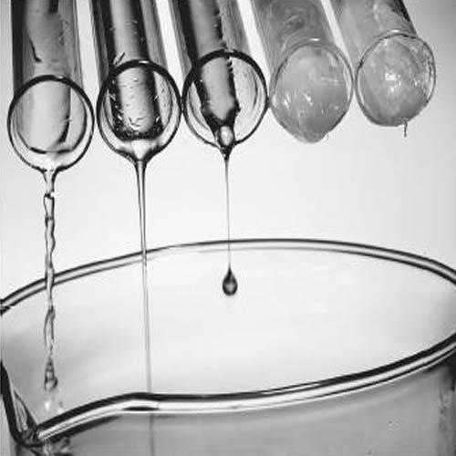
Laminar and turbulent flow

Examples of streamlines in laminar (left) and turbulent (right) flows

Laminar flow

Flow with approximately parallel streamlines. Layers glide by with little mixing or transport across, exchange only occurs by molecular diffusion.

• Regular and predictable.

Turbulent flow

Highly irregular, almost random flow that is very diffusive, with 3D curved streamlines. Can apply over large time and space scales. Dissipative in nature.

• Cannot be predicted deterministically in time or space: requires statistics

All viscous flows can broadly be classified as laminar and turbulent flows, although an intermediate category of transition between the two has also been recognized. A laminar flow is characterized by smooth, orderly, and slow motion in which adjacent layers (laminae) of fluid slide past each other with very little mixing and transfer (only at the molecular scale) of properties across the layers. Turbulent flows are highly irregular, almost random, three-dimensional, highly rotational, dissipative, and very diffusive (mixing) motions. Highly irregular variations (fluctuations) in both time and space (e.g. turbulent fluctuations of velocity in the ABL typically occur over time scales ranging from 10^-3 to 10^4 s and the corresponding spatial scales from 10^-3 to 10^4 m). Due to their nearly random nature, turbulent motions cannot be predicted or calculated exactly as functions of time and space; one usually deals with their average statistical properties. Although there are many examples and applications of laminar flows in industry, in the laboratory, and in biological systems, their occurrence in natural environments, particularly the atmosphere, is rare and confined to the so-called LBL over smooth surfaces (e.g., ice, mud flats, relatively undisturbed water, and tree leaves). Most fluid flows encountered in nature and engineering applications are turbulent. In particular, the various small-scale motions in the lower atmosphere are turbulent. The turbulent mixing layer may vary in depth from a few tens of meters in clear, calm, nocturnal cooling conditions to several kilometers in highly disturbed (stormy) weather conditions involving deep penetrative convection.

Laminar or turbulent?

The flow between the two red lines could best be described as:

• A Turbulent
• B Laminar
• C Anisotropic
• D All of the above

smoke from a smoldering candle in a still room, are laminar initially. The flow is therefore smooth in appearance. The slow flow of water from a laboratory faucet

Effect of flow velocity

As flow speed increases, so does the turbulence Source

Laminar flow, Turbulent flow by Reynolds Experiment Osborne Reynolds demonstrated that there are two distinctly different types of flow by injecting a very thin stream of colored fluid having the same density of water into a large transparent tube through which water is flowing.

Effect of viscosity

Turbulence is easier to create in low viscosity fluids

Turbulence is easier to create in low viscosity fluids, but more difficult in highly viscous fluids.  Turbulence is caused by excessive kinetic energy in parts of a fluid flow, which overcomes the damping effect of the fluid’s viscosity. Laminar flow is characteristic of very slow moving, shallow water, which is uncommon in nature.  It is also characteristic of flows in “fluids” that are very viscous, like glacial ice or mud flows that have little water.

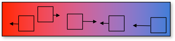
Effect of differential forces

This figure shows how a boundary layer grows with distance over a flat plate. The thickness of the laminar boundary layer grows but eventually a critical combination of properties (speed of flow, distance and viscosity) is exceeded after which the flow breaks down into the haphazard jumble of eddies characteristic of turbulent flow. However, note that a laminar sub-layer still remains at the surface. The thickness of the sub-layer mainly depends upon the roughness of the surface and the external wind speed. Over relatively smooth surfaces, and especially with high wind speeds, the layer becomes very thin or is temporarily absent. The onset of turbulence can be predicted by the Reynolds number, which is the ratio of inertial forces to viscous forces within a fluid Immediately above the surface is the laminar boundary layer (LBL). It is the thin skin (only a few millimeters) of air adhering to all surfaces within which the motion is laminar (i.e. the streamlines are parallel to the surface with no cross-stream component).

Turbulence

Turbulence is a feature of flows, not fluids.

• Turbulent flows are very efficient in equalizing temperature and concentration gradients:

  • In the Atmosphere, turbulent flows are 105 times faster than molecular diffusion.

Turbulence is a feature of fluid flow, not of the fluid. When the Reynolds number is high enough, most of the dynamics of turbulence are the same whether the fluid is an actual fluid or a gas. Most of the dynamics are then independent of the properties of the fluid. Cover cup to prevent cooling!

Turbulent flow is defined as the flow in which the system’s inertial forces are dominant over the viscous forces. This phenomenon is described by Reynolds number, a unit-less number used to determine when turbulent flow will occur.

 

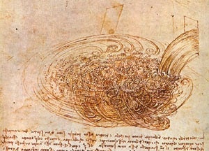
Turbulence

• Eddies are coherent parts within the moving fluid.
• Eddies exist in a wide range of different sizes.
• The smallest eddies dissipate to heat.

Leonardo da Vinci’s famous drawing of water poured into a pot: His turbulent flow superimposes different scales of eddies.

An eddy may be considered akin to a vortex or a whirl in common terminology. Turbulent flows are highly rotational and have all kinds of vortexlike structures (eddies) buried in them. However, eddies are not simple two-dimensional circulatory motions of the type in an isolated vortex, but are believed to be complex, three-dimensional structures. Eddies generally become more numerous as the fluid flow velocity increases. Energy is constantly transferred from large to small eddies until it is dissipated. Turbulent flow consists of a hierarchy of eddies of a wide range of sizes (length scales), from the smallest that can survive the dissipative action of viscosity to the largest that is allowed by the flow geometry. The range of eddy sizes increases with the Reynolds number of the overall mean flow. In particular, for the ABL, the typical range of eddy sizes is 10^-3 (mm) to 10^3 (km).

Properties of turbulence

• Irregular, random, and three-dimensional
  • Motions are rotational and anisotropic
• Diffusive & dissipative
  • Ability to mix properties
  • Energy of motion is degraded into heat
• Consists of multiple length scales
  • Large scales of energy input break down into smaller and smaller scales

“Big whirls have little whirls, That feed on their velocity; And little whirls have lesser whirls, And so on to viscosity.”

― Lewis Fry Richardson

Irregular: This makes any turbulent motion essentially unpredictable. For this reason, a statistical description of turbulence is invariably used in practice. Diffusive: It is responsible for the efficient diffusion of momentum, heat, and mass (e.g., water vapor, CO2, and various pollutants) in turbulent flows. Macroscale diffusivity of turbulence is usually many orders of magnitude larger than the molecular diffusivity. Dissipative: The kinetic energy of turbulent motion is continuously dissipated (converted into internal energy or heat) by viscosity. Therefore, in order to maintain turbulent motion, the energy has to be supplied continuously. If no energy is supplied, turbulence decays rapidly. Multiple length scales: All turbulent flows are characterized by a wide range (depending on the Reynolds number) of scales or eddies. The transfer of energy from the mean flow into turbulence occurs at the upper end of scales (large eddies), while the viscous dissipation of turbulent energy occurs at the lower end (small eddies).

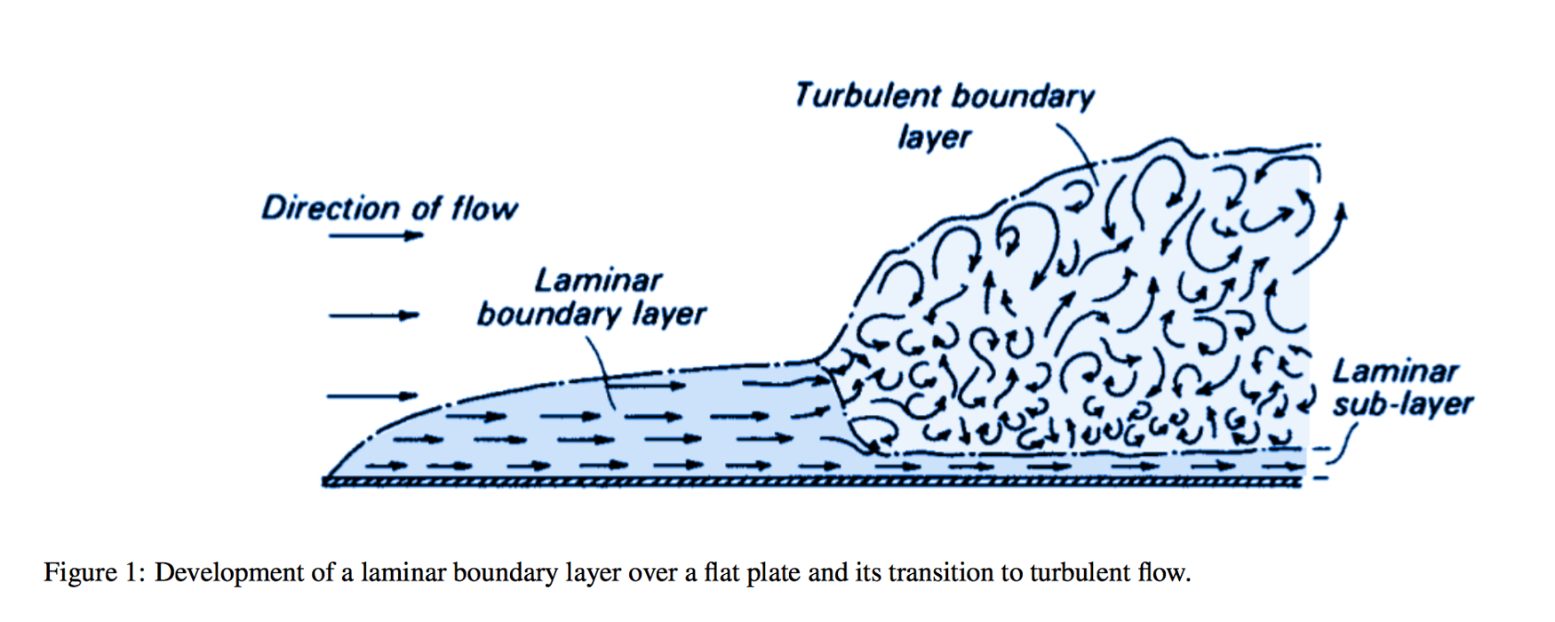
Visualizing the LBL

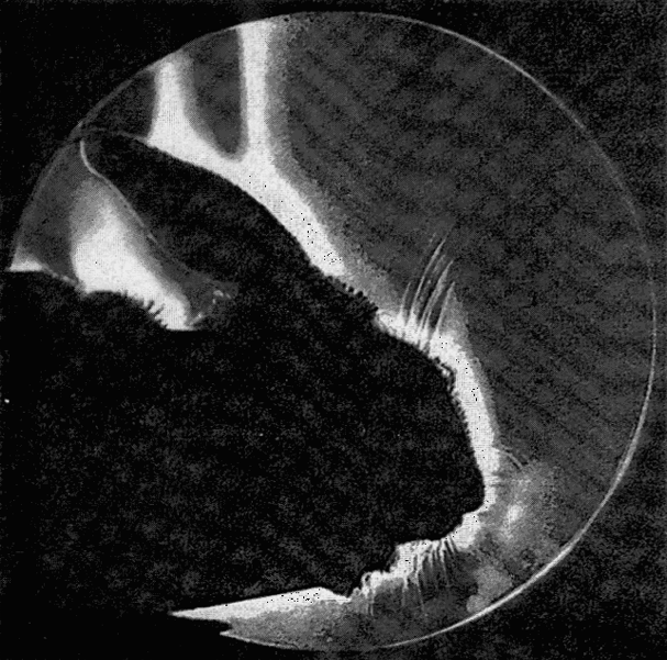
The LBL can be made visible using the Schlieren photography. This technique uses the temperature dependence of the index of refraction of air.

Schlieren photograph of rabbit’s head (cooler air: dark, warmer air: light)

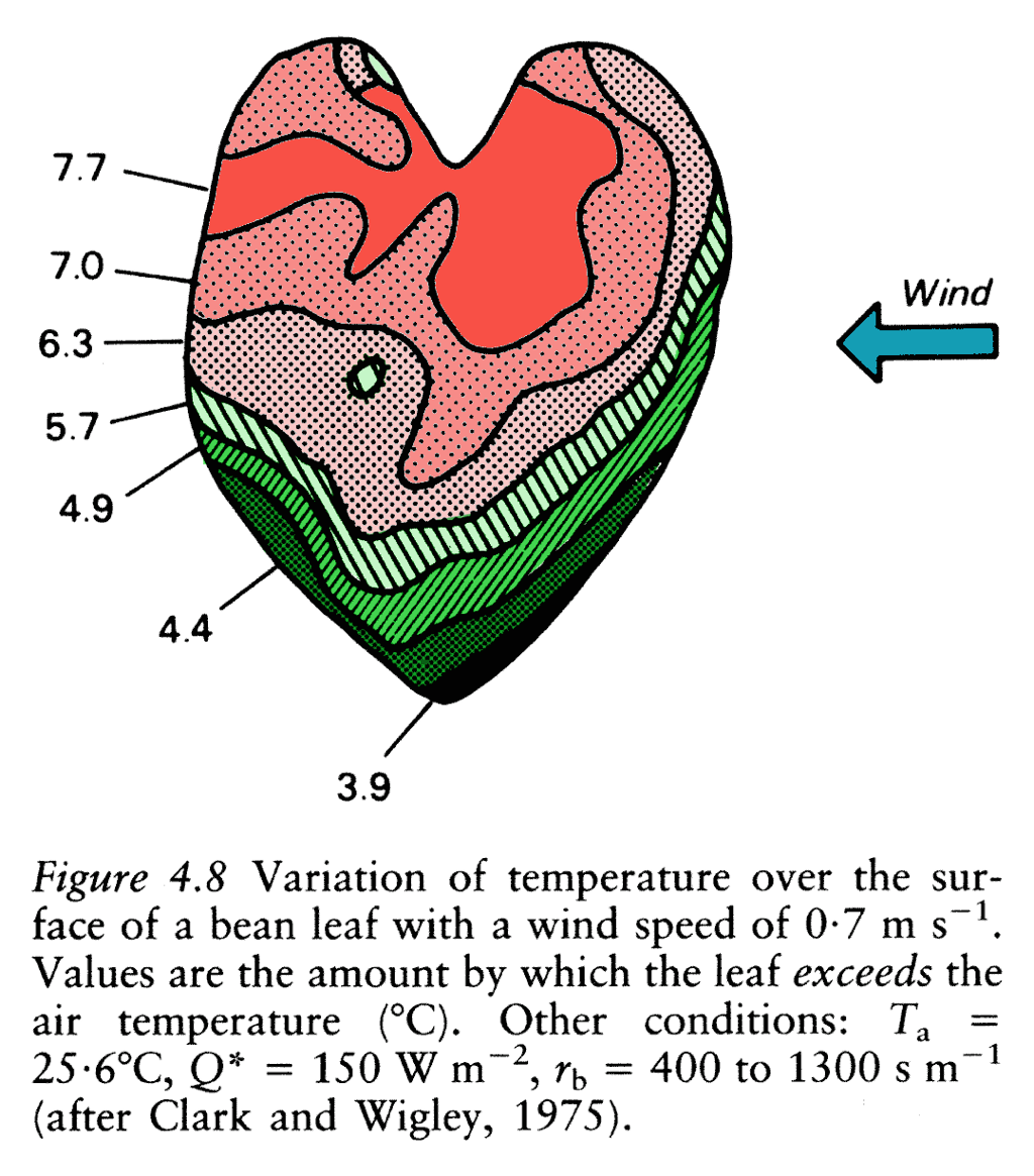
The laminar boundary layer (LBL)

This thin layer (5 to 50 mm) is very important.

• It adheres to all objects and because diffusion is very poor (molecular) it provides a buffer between the object and the turbulent air above.

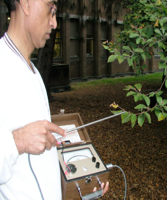
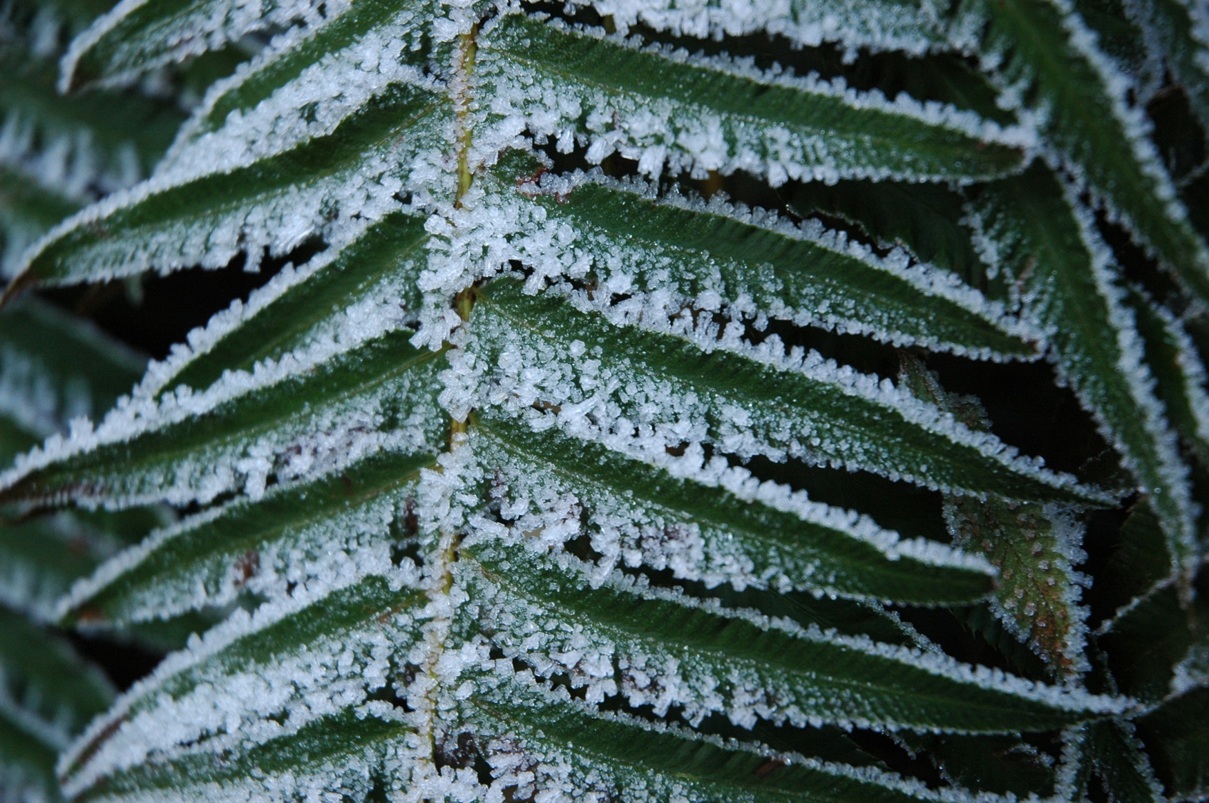
Measurements in the LBL of leaves with a hotwire probe (Photo: R. Jassal, UBC).

Immediately above the surface is the laminar boundary layer (LBL). It is the thin skin (only a few millimeters) of air adhering to all surfaces within which the motion is laminar (i.e. the streamlines are parallel to the surface with no cross-stream component). The connotation is that adjacent layers (laminae) of the fluid remain distinct and do not intermix.

Importance of the LBL

• The principles we’ll learn about the LBL are important in developing formulae for calculating:
  • rates of transpiration and evaporation from leaves
  • rates of CO2 uptake by leaves (plant growth)
  • rates of pollutant (O3, SO2) deposition on leaves
  • rates of heat loss from buildings, humans, & animals

Sulfur dioxide

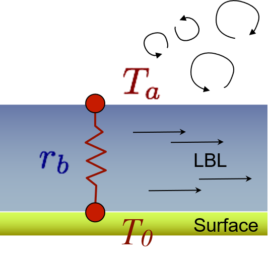
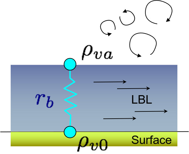
Describing exchange in the LBL

Fluxes that pass through the LBL (molecular transport) are proportional to gradients between surface and turbulent atmosphere.

Sensible heat

\(H\propto K_H\small\frac{\delta T}{\delta z}\)

• \(K_H\) molecular diffusivity for heat

Latent heat

\(LE\propto K_{LE}\small\frac{\delta \rho_v}{\delta z}\)

• \(K_{LE}\) molecular diffusivity for water vapor

Momentum

\(\tau\propto K_{M}\small\frac{\delta u}{\delta z}\)

• \(K_M\) molecular diffusivity for momentum

In the laminar sublayer there is no convection molecular diffusion coefficients = molecular diffusivity in m2 s^-1. K values are very small, of the order of 10^-5 m2 s^-1, thus providing an important insulating barrier between the surface and the bulk of the atmosphere. Fick’s Law of diffusion! Momentum, same as ‘Shear stress’ (stress that results from layers moving past each other) – in the surface layer of frictional influence generates this shearing force and transmits it downwards as a flux of momentum. Thus the gradients of climatic properties (T, water vapor, [CO2], u, etc.) are very steep in the LBL, and since both the flux and the diffusivity are constant with height the vertical profile of a property is approximately linear, i.e. the gradient is constant.

Describing heat exchange in the LBL

Ohm’s law (resistance) format very useful:

\[ H = \small\frac{C_a(T_0-T_a)}{r_b} \qquad(2)\]

• Where \(r_b\) is the boundary layer resistance in s m^-1 which mainly depends on thickness of the LBL.

Ohm’s Law  Current = V/R

Characteristics of the LBL

Why this temperature distribution? Thickness of LBL depends on:

• Object size, shape, orientation, and roughness
• Inversely on wind speed & turbulence intensity

T.R. Oke (1987): ‘Boundary Layer Climates’ 2nd Edition, with permission.

Weak but turbulent air Temperature difference increases from the windward to the leeward side since the LBL increases with distance from edge of leaf

Latent heat exchange in the LBL

Fick’s Law of diffusion can be written in resistance form for the transfer of water vapour (latent heat) in the LBL:

\[ LE = \small\frac{L_v(\rho_{v0}-\rho_{va})}{r_b} \qquad(3)\]

Where \(r_b\) is again the boundary layer resistance for water vapour in s m^-1

Fick’s Law of diffusion - molecular diffusivity

Why does the frost accumulate at the edge of the leaf?

Photo by A. Christen

The thinner LBL at the edge accumulates more frost because of a better \(LE\) exchange (lower \(rb\))

Photo by A. Christen

Take Home Points

• A laminar flow has approximately parallel streamlines. Layers glide by. A turbulent flow is highly irregular, and contains many scales of eddies.
• Turbulent and laminar are properties of the flow, not the fluid.
• Within millimetres of the surface of objects, the flow is always laminar - this is the laminar boundary layer (LBL)
• Molecular transfer of energy (heat) and mass in the LBL can be described using resistances in analogy to Ohm’s law.