Modelling Sub-Surface Temperatures

Modelling Sub-Surface Temperatures

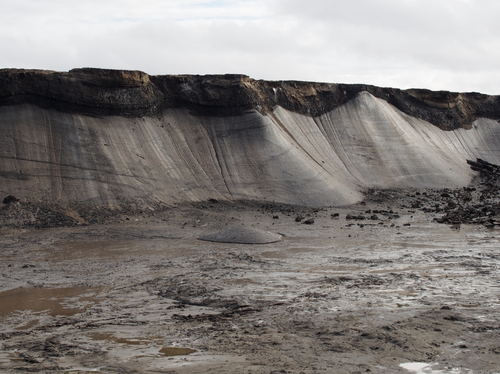
High Arctic Landscape on Fosheim Peninsula, Ellesmere Island - a rapidly warming Arctic causes permafrost thawing and mass movements (Photo: A. Cassidy)

Learning Objectives

• Describe how can we predict soil temperature using a selected solution to the heat conduction equation.
• Explain how soil temperature waves move in soils.

Photo: A. Cassidy

The course of soil temperature at a particular depth Tz with time is very regular in comparison with almost any other atmospheric element.

Learning Objectives

• How do substrate temperatures change on diurnal and annual scales?
• Can we predict timing and amplitude of soil temperature waves using a selected solution to the heat conduction equation.
• How can we alter substrates to control soil thermal climates (agriculture, design)?

A rapidly warming Arctic causes permafrost thawing and mass movements (thaw slump) Undisturbed areas Permafrost scar Newly exposed areas Other examples – agriculture, modeling the global C cycle, global biogeochemical cycles - lots of reasons we would want to be able to understand and predict soil T.

Year-long thaw-slump temperatures

A rapidly warming Arctic causes permafrost thawing and mass movements (thaw slump) Undisturbed areas Permafrost scar Newly exposed areas Other examples – agriculture, modeling the global C cycle, global biogeochemical cycles - lots of reasons we would want to be able to understand and predict soil T.

Source

Sub-Surface Temperature Profile

Idealized soil temperature profile in summer

The course of soil temperature at a particular depth Tz with time is very regular in comparison with almost any other atmospheric element. What direction is our soil heat flux? Geothermal gradient is the rate of increasing temperature with respect to increasing depth in the Earth’s interior. The Earth’s internal heat comes from a combination of residual heat from planetary accretion, heat produced through radioactive decay, latent heat from core crystallization, and possibly heat from other sources.

Sub-Surface Temperature (iClicker)

What direction is the soil heat flux (QG) at the surface?

• A Downward (+)

• B Upward (-)

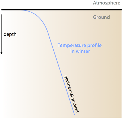
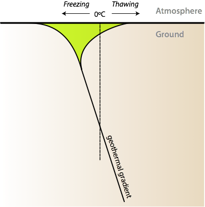
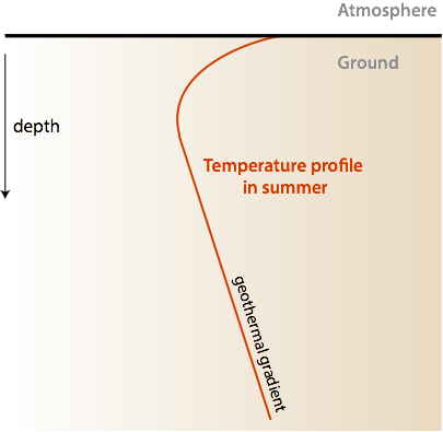
Sub-Surface Temperature Profile

Idealized soil temperature profile in winter

Sub-Surface Temperature Profile

the annual wave may penetrate to about 14 m

Sub-Surface Temperature Profile

The temperature at this depth is sometimes used as a surrogate for the average annual air temperature of the site.

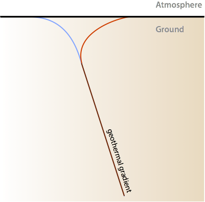
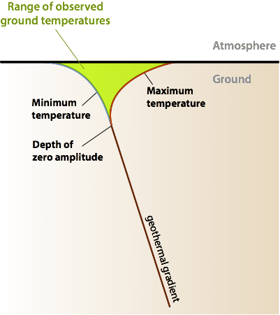
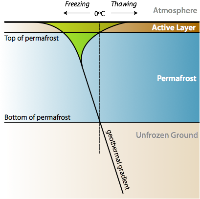
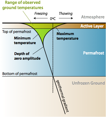
Permafrost Temperature Profile

Permafrost Temperature Profile

Permafrost Temperature Profile

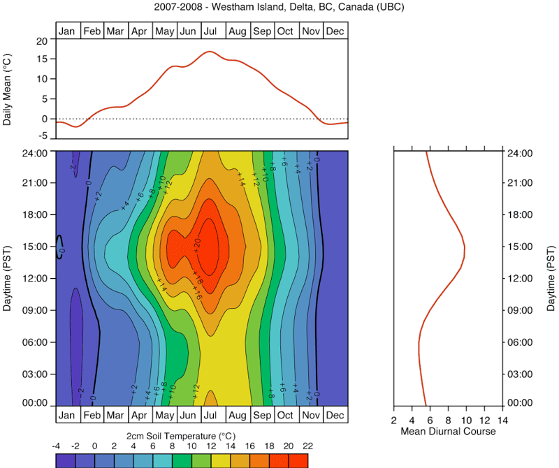
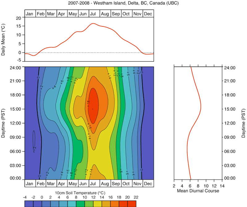
Sub-Surface Temperature Variability

Westham Island, 2cm depth

Sub-Surface Temperature Variability

Westham Island, 10cm depth

amplitude decreases exponentially. phase shift (time lag) increases linearly.

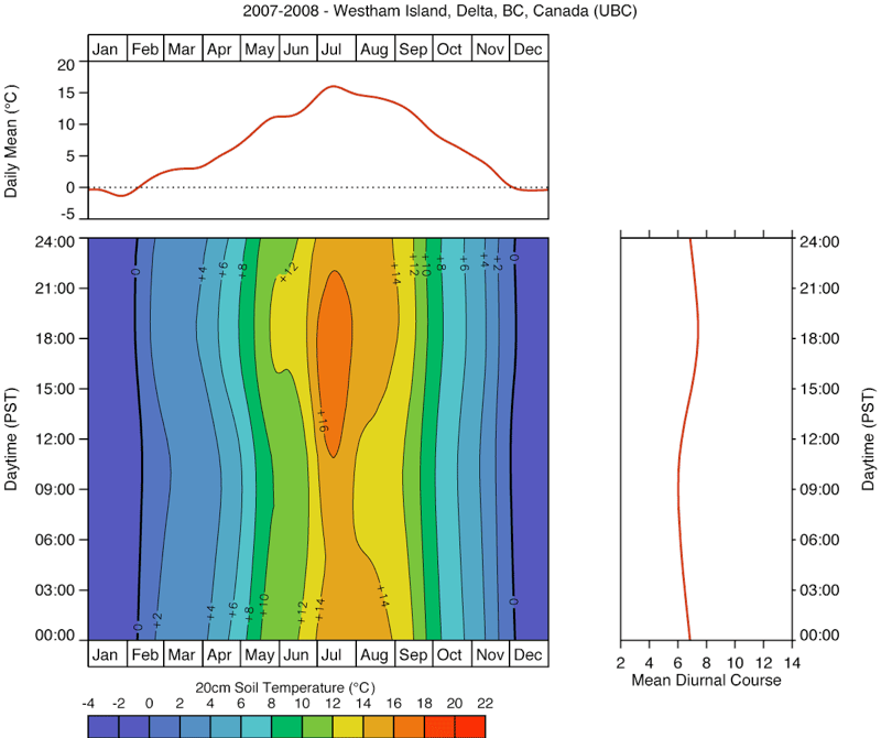
Sub-Surface Temperature Variability

Westham Island, 20cm depth

amplitude decreases exponentially. phase shift (time lag) increases linearly.

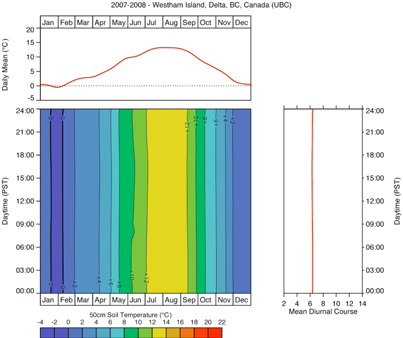
Sub-Surface Temperature Variability

Westham Island, 50cm depth

amplitude decreases exponentially. phase shift (time lag) increases linearly.

Soil Temperature Waves

Surface wave moves down in response to radiative forcing at different periods \(P\)

• annual (1 year) to ~14 m
• daily (1 day) to ~0.75 m
• cloud passage (~15 min) to ~0.1 m

Wave amplitude and phase shift (time lag) with depth:

• amplitude decreases exponentially
• phase shift increases linearly

Draw temperature profile with depth

Soil Temperature Waves

The daily and annual periodic forcing by the sun creates a surface temperature (\(T_o\)) wave, which propagates into the soil below. If we make the following assumptions:

1. The thermal diffusivity κ = k/C is uniform
2. Cycles are sinusoidal (better for year than day)

Then then \(T_o\) at time \(t\) (in seconds) over period \(P\) can be approximated as:

\[ T_{(o,t)}=\overline{T_o}+\Delta T_o \sin(\omega t) \qquad(1)\]

where \(\overline{T_o}\) is the mean surface temperature over \(P\), \(\Delta T_o\) is the wave amplitude (\(\small\frac{1}{2}\) range of \(T_o\)), and the angular frequency of oscillation is \(\omega = 2\pi / P\).

kappa = It tells us how fast a temperature wave will diffuse or travel downward into a soil Trigonometry sinusoidal daily course the angular frequency = scalar measure of rotation rate Larger P, lower the angular frequency; higher P, greater than angular frequency

Calculate the Angular Frequency (iClicker)

Annual \(\omega_a\)

# Number of seconds in a year
P = 60 * 60 * 24 * 365.24 
# Solve
omega_a = 2*pi/P
sprintf('Angular Frequncy of a year %0.3e s-1',omega_a)

[1] "Angular Frequncy of a year 1.991e-07 s-1"

Daily \(\omega_d\)

Which value give the closest approximation of \(\omega_d\)?

• A 3.636e-05 s-1
• B 1.454e-04 s-1
• C 7.272e-05 s-1
• D 1.991e-07 s-1

Analytical solution for sinusoidal forcing.

Checkout this resource to see some animated plots.

A solution of Fourier’s heat conduction. file:///Volumes/sknox01/Teaching/GEOB300/Website/geob300/applets/stwave/index.html

A Solution of Fourier’s Heat Conduction

With the surface temperature wave equation as the boundary condition, we can find an analytic solution to the Fourier heat conduction equation in 1-D:

\[ T_{(z,t)}=\overline{T_o}+\Delta T_o e^{-z(\small\frac{\omega}{2K})^{1/2}} \sin(\omega t - (\small\frac{\omega}{2K})^{1/2}z) \qquad(2)\]

• exponential term: Wave amplitude at depth z relative to the surface temperature wave
• sine function: Phase shift of the wave at depth z

Note: the wave decays exponentially with depth, and the decay is less in soils with large κ, or if the period is longer.

Boundary conditions (b.c.) are constraints necessary for the solution of a boundary value problem. They are a set of additional constraints. Omega = angular frequency thermal diffusivity = how fast a temperature wave will diffuse or travel downward into a soil

Damping Depth

The inverse of the exponential term defines a useful feature, the damping depth (\(D\)).

• It is the depth at which the surface temperature wave is reduced to \(e^{-1}\) (37%) of its value at z = 0.
• At 3D it drops below 5%, and 4.6 D below 1%.

\[ D = \sqrt{\small\frac{2K}{\omega}} = \sqrt{\small\frac{KP}{\pi}} \qquad(3)\]

The red line is the surface temperature range \(2 \Delta T_o\). Blue is the temperature range at depth \(D\); \(0.37 2 \Delta T_o\)

In most soils the daily surface temperature wave is only discernible to a depth of about 0.75 m. In soils with low κ values it is even less, indicating that flux convergence has extinguished QG in a thin near-surface layer. thermal diffusivity = how how fast a temperature wave will diffuse or travel downward into a soil

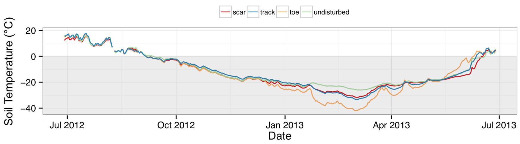
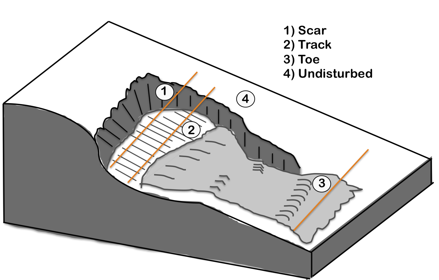
Example - Effect of Organic Cover

thermal diffusivity = how fast a temperature wave will diffuse or travel downward into a soil Note, the wave decays exponentially with depth, and the decay is less in soils with large κ, or if the period is longer.

Phase Shift - Max and Min Soil Temperatures

Term 2 of the 1-D analytical solution (Equation 2) gives the phase shift equation for features such as maximum and minimum soil temperatures, which occurs at 0.5 π and 1.5 π, i.e.:

• \(\sin(\omega t - (\small\frac{\omega}{2K})^{1/2}z) = \pm 1\)

Solving for \(t\) gives:

\(\Delta t_m = t_{m_2} - t_{m_1} = (z_2 - z_1)(\small\frac{1}{2\omega K})^{1/2}\)

\(\Delta t_m\) is the phase shift; \(t_{m_1}\) and \(t_{m_2}\) are times at which maximum or minimum soil temperatures occur at \(z_1\) and \(z_2\) respectively.

The time lag (phase shift) for the wave crest (maximum) and trough (minimum) to reach lower depths is given by where t1 and t2 are the times at which the wave crest or trough reaches depths z1 and z2.

Phase Shift (iClicker)

When will soil temperature reaches its maximum at 5 cm if the maximum surface temperature is measured at 13:00? Assume a thermal diffusivity K = 5.0×10−7 m² s⁻¹.

• A 5863.2301428
• B 14.628675
• c 14:38

Breakout groups

Phase shift (Implications)

• The phase shift at a certain depth is least in soils with large κs.
• These idealized patterns are disrupted by:
• Variable cloud cover.
• Rain (percolation gives wetting front).
• Freezing/melting (latent heat effects).
• Snow cover (insulates).
• Soil inhomogeneities in the horizontal and vertical.

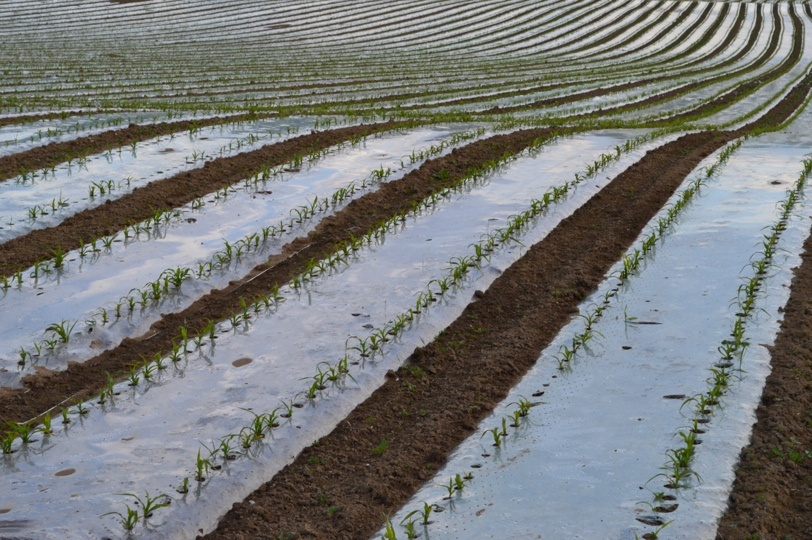
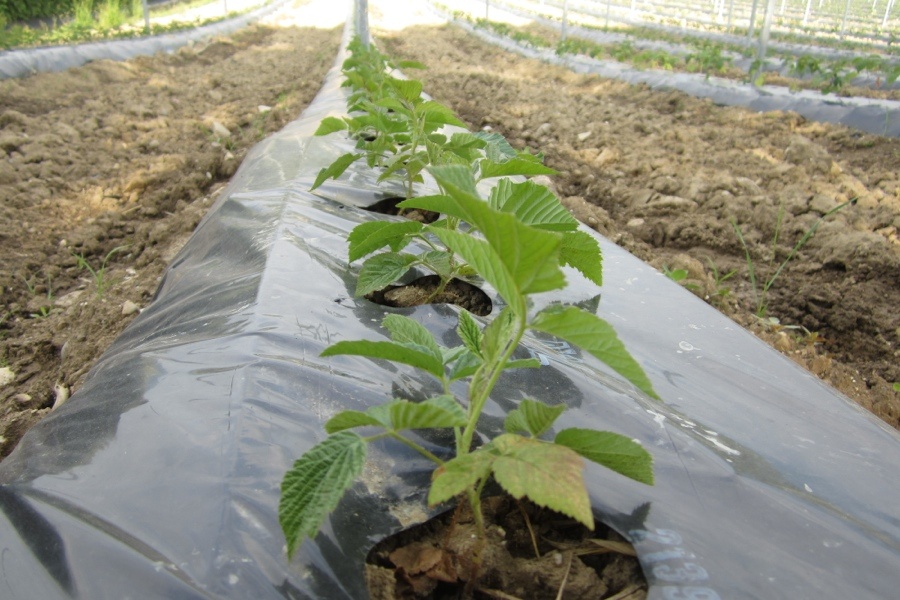
Modification and Control of Soil Climates

Relatively little can be done economically to modify the external forcing (shade is an exception). But the nature of the soil can be manipulated.

• Albedo - surface dressing with dark or light-cultured materials.
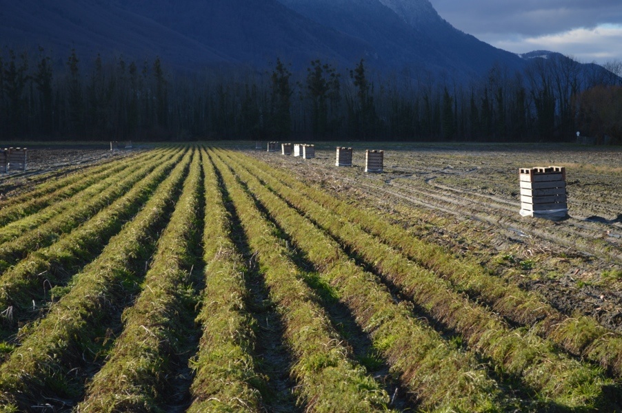
• Ridge and furrows - control surface geometry to maximize or minimize K* and L* and surface moisture state.
• Moisture - wetting or drainage can greatly alter thermal properties.
• Compaction / cultivation - control of air content and its role in thermal properties.

Ridge and Furrow Geometry

The furrow and ridge geometry enhances the irradiance of solar radiation on the sloped sides The furrow and ridge geometry enhances shortwave absorption by decreasing the system albedo (multiple reflection) The furrow and ridge geometry reduces long-wave loss by L∗ due to a reduced sky view factor

Modification and Control of Soil Climates

• Stripping surface cover - remove organic layer, snow cover, vegetation cover.
• Mulches - introduce layer of insulation (straw, leaves, husks, foam)

Photo: A. Christen

Photo: A. Christen

Reasons for applying mulch include conservation of soil moisture, improving fertility and health of the soil, reducing weed growth and enhancing the visual appeal of the area. Some research has been done using different colors of mulch to affect crop growth. 

Heat Sharing

The partitioning of total ‘sensible’ heat flux between the soil (\(H_g\)) and the atmosphere (\(H\)).

\[ \frac{H_g}{H} = \frac{\mu_g}{\mu_a} \qquad(4)\]

• Soil and atmosphere share in accepting heat during daytime and releasing heat at night. \(\mu_g\) and \(\mu_a\) are the soil and atmospheric thermal admittance respectively.

  • \(\mu_a\) increases with wind speed and convection (mixing).

Take home points

• We observe temperature waves with annual, diurnal and even short-term (cloud-passage) periods.
• In a uniform soil, the wave amplitude decays exponentially, whereas the phase-shift is linear with depth.
• The damping depth is a commonly used term to quantify the depth to which 37% of the surface amplitude reaches down.

Heat conduction equation