Soil Thermal Properties

Today’s learning objectives

• Provide examples of why processes in the ground are of interest to climatologists.

• Discuss key properties that describe the thermal behavior of the surfaces in the climate system.
• Explain how the key properties relate to heat conduction in soils.

Discussion (iClicker)

Why might climatologists be interested in studying soil thermal properties and subsurface processes?

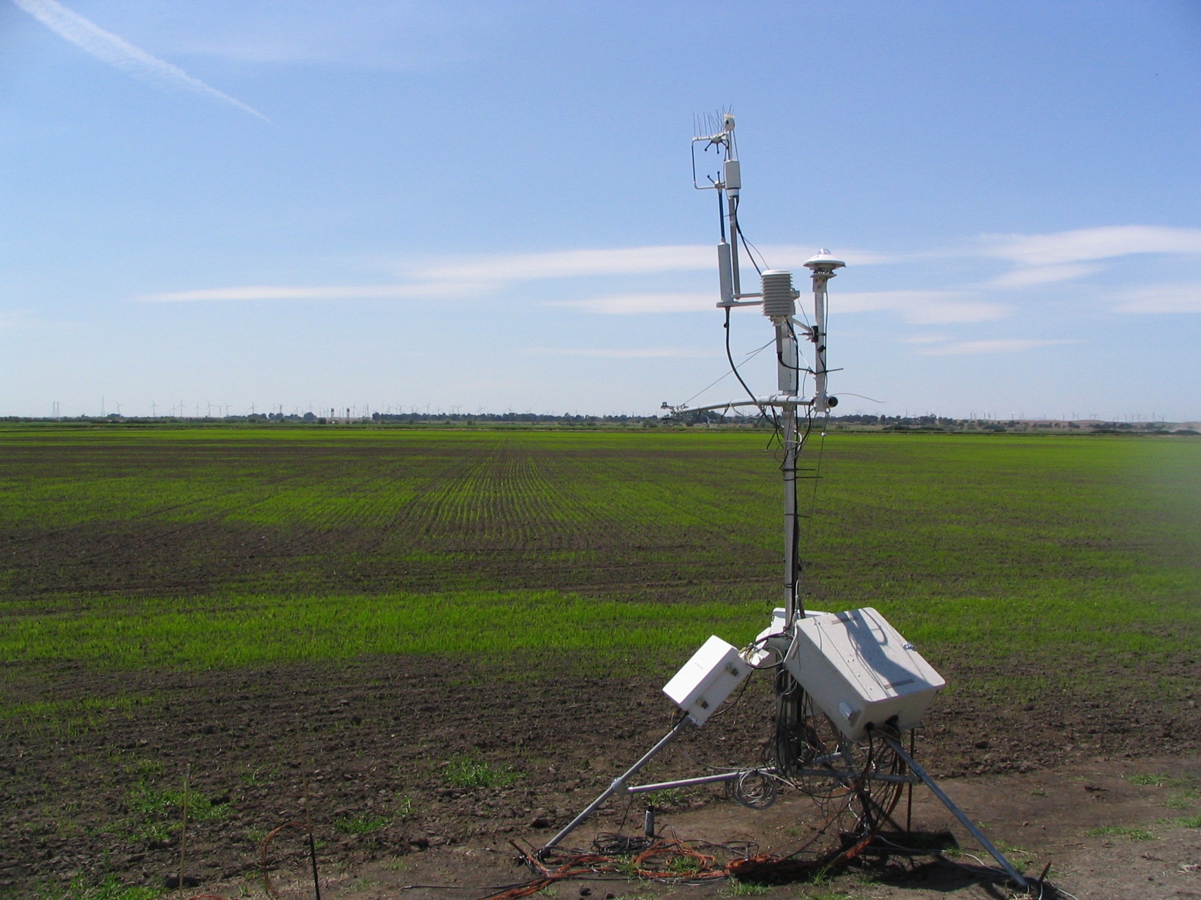
Agriculture

Soil temperatures directly impact germination and growth of plants

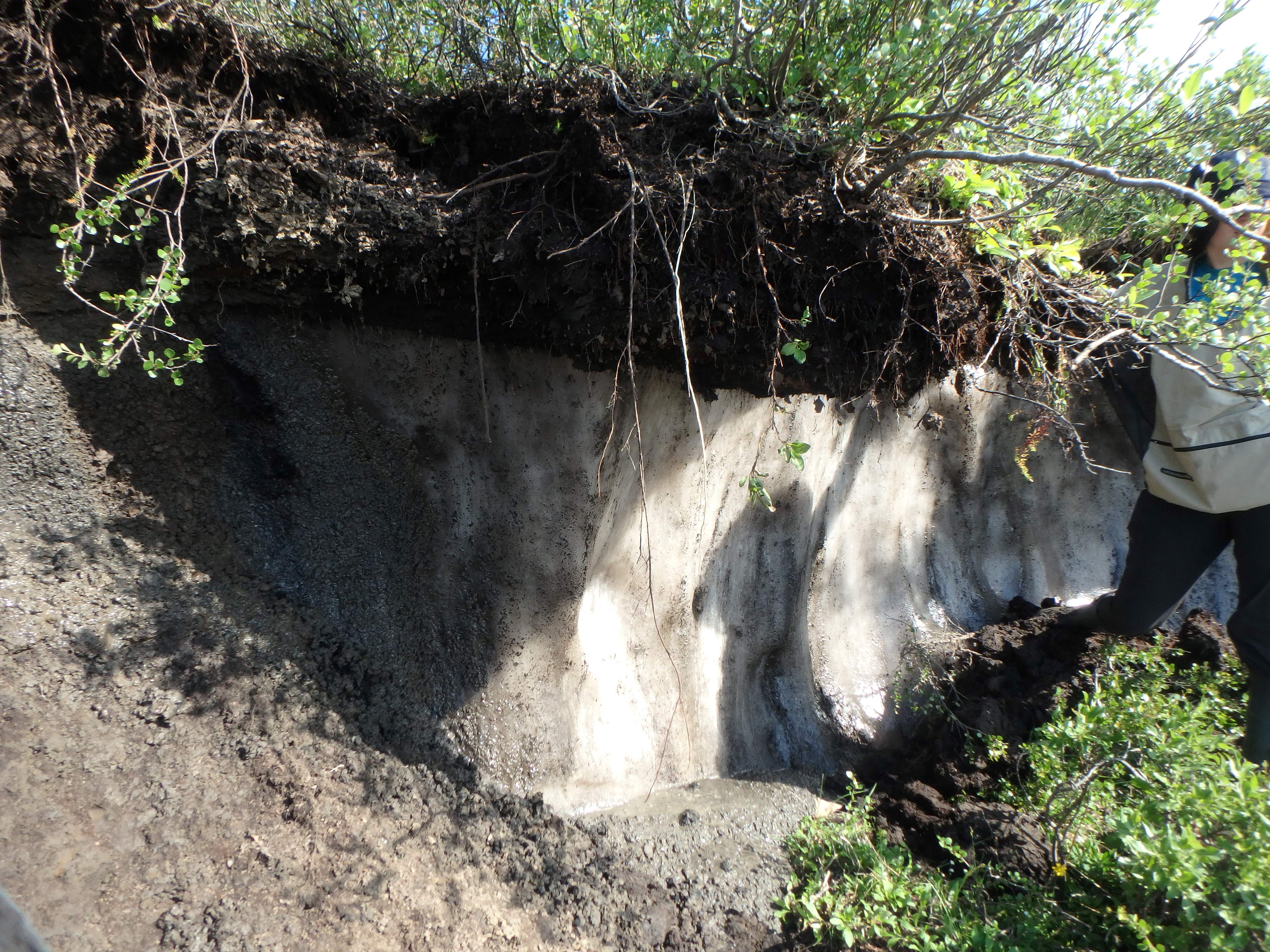
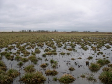
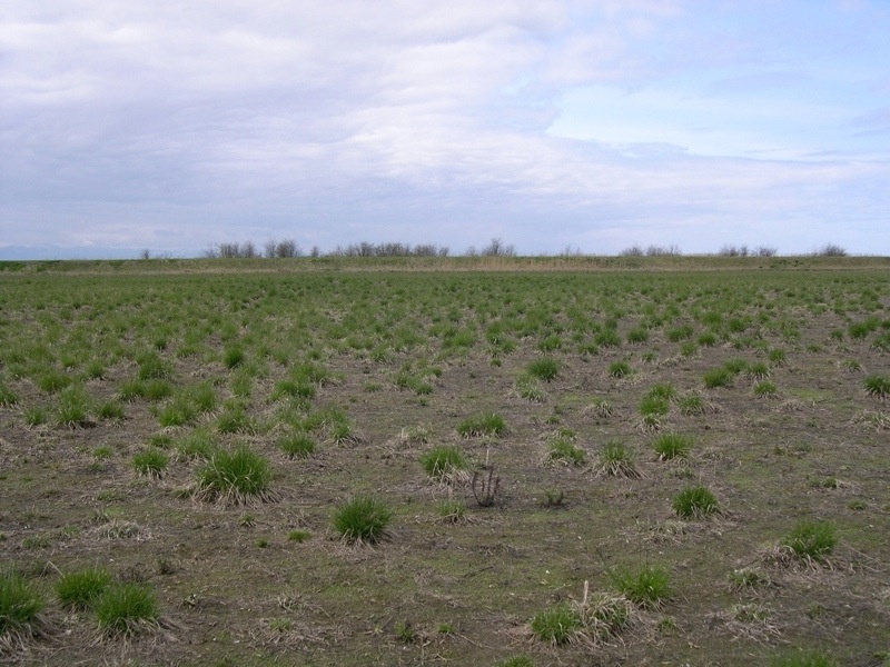
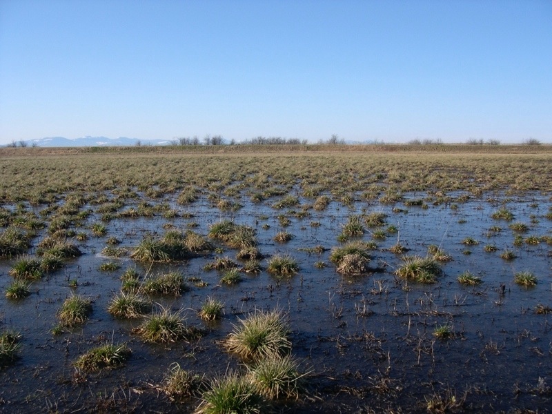
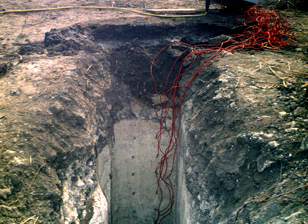
Thermokarst

Melting ground ice, Tuktoyaktuk coastlands, 2017

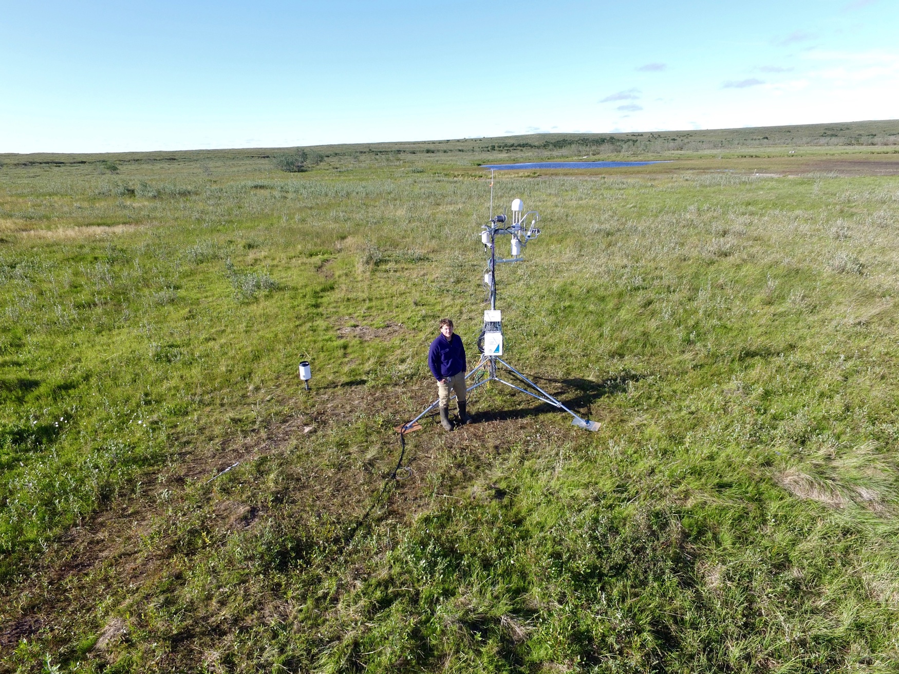
Carbon Storage

Soils can act as a carbon sinks or sources

Role of Soil in the Climate System

The “active” layer of surface extends down to a relatively shallow depth.

• The properties this layer make \(\Delta S\) of sensible heat and water significant over diurnal and annual scales.
• Soils act as a ‘battery’ of both energy and mass relevant effecting the atmosphere.

Because the active surface is the site of greatest energy absorption by day and depletion by night, it is also where the greatest thermal response is found. The effects diminish with distance away from the interface down into the substrate. The surface energy balance causes a temperature wave that establishes a temperature gradient ∂T/∂z and a sensible heat flux QG directed downwards by day and upwards at night. The size of both, ∂T/∂z and QG, diminish with distance away from the interface giving a changing vertical distribution (profile) of substrate temperatures Soil temperatures vary less rapidly than air temperatures, and since radiative and convective exchanges are virtually absent in the soil, most of the activity takes place from molecule to molecule.

Thermal Inertia

Specific heat \(c\): the quantity of heat required to raise the temperature of a unit mass of a material by 1 K.

• Given in J kg^-1 K^-1.

Heat capacity \(C\) is the quantity of heat required to raise the temperature of a unit volume of a material by 1 K.

• Given in J m^-3 K^-1.

The actual rate mean temperature change of a soil layer over time ∆T /∆t is proportional to the amount of heat currently absorbed by the layer (∆Q) but it also depends on the thermal properties of the soil. Let’s discuss some key SOIL THERMAL PROPERTIES

\(C\) and \(c\) of soil materials

Table 1: Heat caqacity and specific heat of selected substances

Material	Heat capacity C MJ m-3 K-1	Specific heat c kJ kg-1 K-1	Density ρ Mg m-3
Air	0.0012	1.01	0.0012
Water (liquid)	4.1800	4.18	1.0000
Ice	1.9000	2.10	0.9000
Mineral soil	2.1000	0.80	2.6500
Organic soil	2.5000	1.90	1.3000
Rock	2.0000	0.80	2.7000

Heat capacity (C) relates to the ability of a substance to store heat and expresses the temperature change produced as a result of gaining or losing heat Where it is clear that, compared to most other materials, water requires a large heat input to effect a given change in temperature whereas air requires very little. C = c*density The value of C for a soil can be calculated by evaluating the fractions of soil solid, water and air.

Volume Fractions and Porosity

\[ \theta_a+\theta_w+\theta_g = 1 \qquad(1)\]

Where \(\theta_a\), \(\theta_w\), and \(\theta_g\) are fractional volumetric contents of soil grains, water, and air respectively. We can then define porosity \(\theta_P\) as: \[ \theta_P = \theta_a + \theta_w = 1 - \theta_g \qquad(2)\]

It is also helpful to further partition soil into mineral \(\theta_m\) and organic \(\theta_o\) fractions:

\[ \theta_g = \theta_m + \theta_o \qquad(3)\]

Volume Fractions and Porosity

Given a sample of know volume and mass, we can determine the fractional composition by:

• Oven-drying soil samples to get \(\theta_w\)
• Burning the dried sample in a furnace to get \(\theta_o\)
• The residual will give us \(\theta_m\)

Bulk Density

Given a “wet” soil sample of know volume (\(V\)) and mass (\(M\)), we can calculate it’s “wet bulk density” \(\rho_w = \frac{M}{V}\).

• Upon drying the sample, we can re-weigh the sample to get it’s dry mass (\(M_{dry}\)), i.e., the mass of all the soil grains.
  • W can then get its “dry bulk density” \(\small\rho_{dry} = \frac{M_{dry}}{V}\), where \(V\) is fixed to the original value.
  • Porosity will be inversely related to \(\rho_{dry}\)
    • Higher \(\rho_{dry}\) means lower \(\theta_P\) and vice versa.
• Upon firing the sample, you can get the mass fractions of mineral \(M_m\) and organic \(M_o\) to determine the % organic content

Compound substances

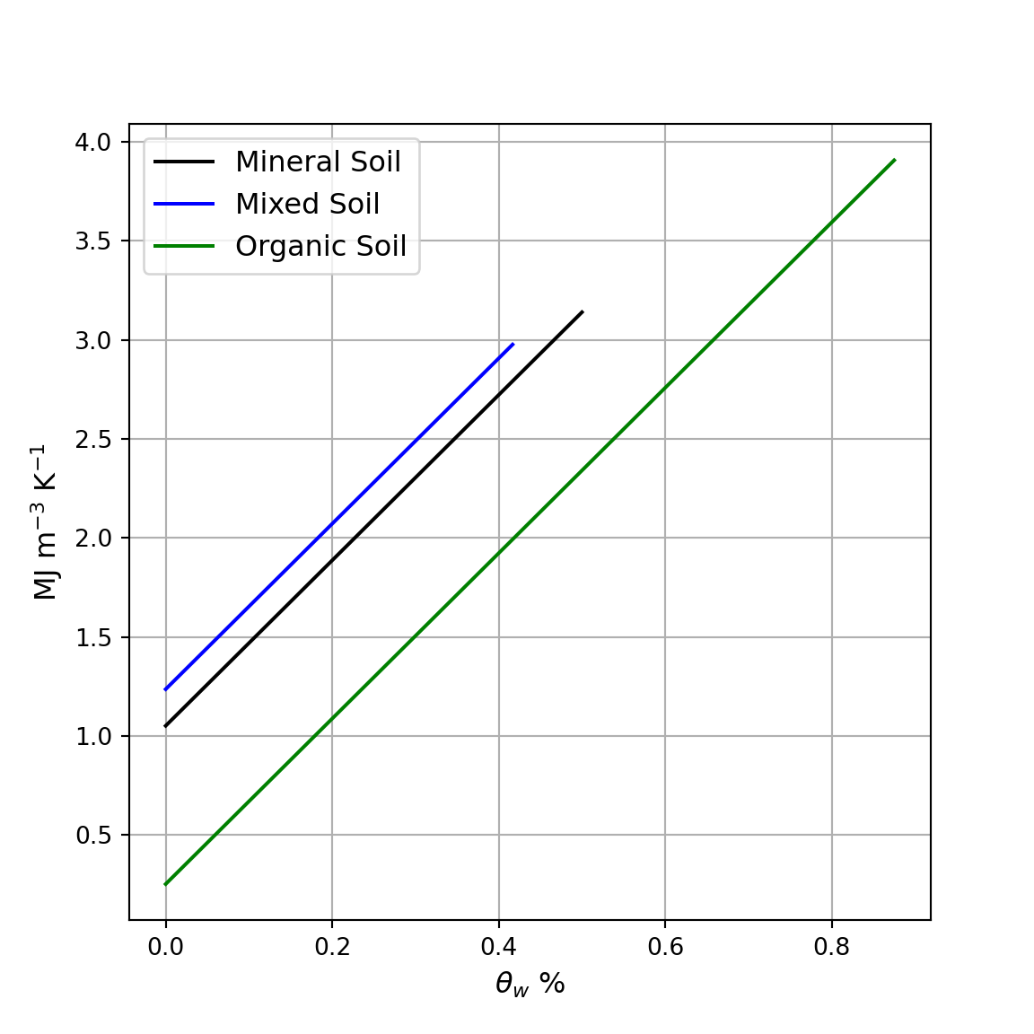
The heat capacity of a mixture of substances such as soil can be calculated if the heat capacity and volume fraction of each component are known. In the case of soil:

\[ C_{s}=C_{m}\theta_{m}+C_{o}\theta_{o}+C_{w}\theta_{w}+C_{a}\theta_{a} \qquad(4)\]

Which example would have the lowest heat capacity?

a.

b.

c.

Figure 1: Three photos of the same location under different conditions.

For example, a wet soil (high C) has a ‘conservative’ thermal climate (it responds sluggishly to heat input or output). Conversely a dry soil (low C) is ‘flashy’ becoming relatively hot by day and cold by night.

Heat capacity vs. Soil Moisture

import numpy as np
import matplotlib.pyplot as plt

def get_C(theta_m,theta_o,theta_w):
    C_w,C_m,C_o,C_a = 4.18, 2.1,2.5,0.0012 # MJ m-3 K-1
    theta_a = 1-(theta_m+theta_o+theta_w)
    theta_a[np.where(theta_a<0)]=np.nan # <<<<<< What does this line do?
    C = C_m*theta_m + C_o*theta_o + C_w*theta_w + C_a*theta_a
    return(C)

theta_w = np.linspace(0,1,25)
C_mineral = get_C(.5,0,theta_w)
C_mixed = get_C(.35,.2,theta_w)
C_organic = get_C(0,.1,theta_w)

What does line 7 in the above codeblock do?

• A: limits \(C\) to plausible values because volumetric fractions cannot be negative
• B: limits \(C\) to plausible values because volumetric fractions cannot sum to more than one

Slope = heat capacity of water Offset = related to porosity

Heat capacity and soil water content

• What is the slope of the line?
• What explains the offset between the lines?

theta_w = np.linspace(0,1,25)
plt.figure(figsize=(6,6))
plt.plot(theta_w,get_C(.5,0,theta_w),color='black',label='Mineral Soil')
plt.plot(theta_w,get_C(.35,.2,theta_w),color='blue',label='Mixed Soil')
plt.plot(theta_w,get_C(0,.1,theta_w),color='green',label='Organic Soil')
plt.ylabel(r'MJ m$^{-3}$ K$^{-1}$',fontsize=12)
plt.xlabel(r'$\theta_w$ %',fontsize=12)
plt.grid()
plt.legend(fontsize=12)

Relationship between C and VWC, try the code out yourself to explore the relationship further

Slope = heat capacity of water Offset = related to porosity

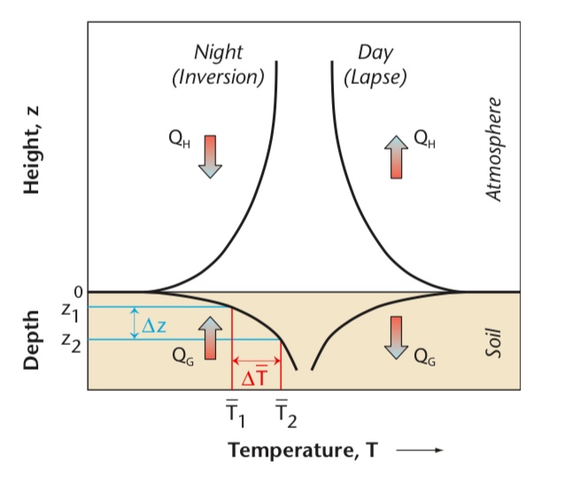
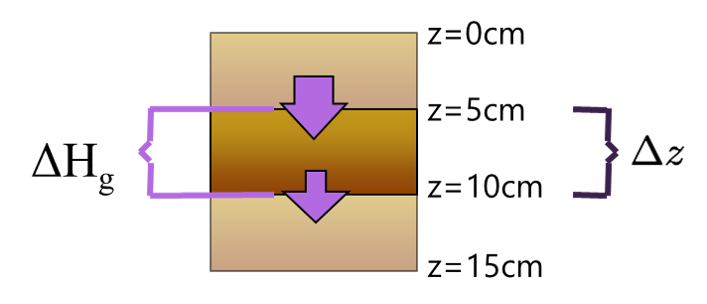
Soil Heat Flux

The flux of heat energy through a given soil layer (\(\frac{H_g}{z}\)) is a product of the layers heat capacity \(C\) and it’s rate of temperature change with time (\(\frac{\Delta T_s}{t}\)):

\[ \frac{H_g}{z} = C_{s} \frac{\Delta T_{s}}{\Delta t} \qquad(5)\]

• Why do we need to consider \(H_{g}\) on a per-layer (\(z\)) basis?

Soil Heat Flux (iClikcer)

C_s_g = 2 #MJ m-3 K-1
Delta_T = 1 #K
Delta_t = 3600 #s (1 hour)
z = 0.01 #m (1 cm)

H_g_z = C_s_g*Delta_T/Delta_t*z

Evaluating the above code give a value of: 0.000 W m^-2 Does this appear correct?

• A True
• B False

Heat Flux Divergence

If we know the heat flux at the top and bottom of some soil layer, we can calculate the change in temperature over the layer as:

\[ \small\frac{\Delta T_s}{\Delta t} = -\small\frac{1}{C_s}\small\frac{\Delta H_g}{\Delta z} \qquad(6)\]

where: \(\small\frac{\Delta H_g}{\Delta z} = \small\frac{H_{g(z_2)}-H_{g(z_1)}}{z_2-z_1}\)

• \(\Delta H_g\) is the heat flux divergence term
  • It is the energy that goes into (or is released from) the layer

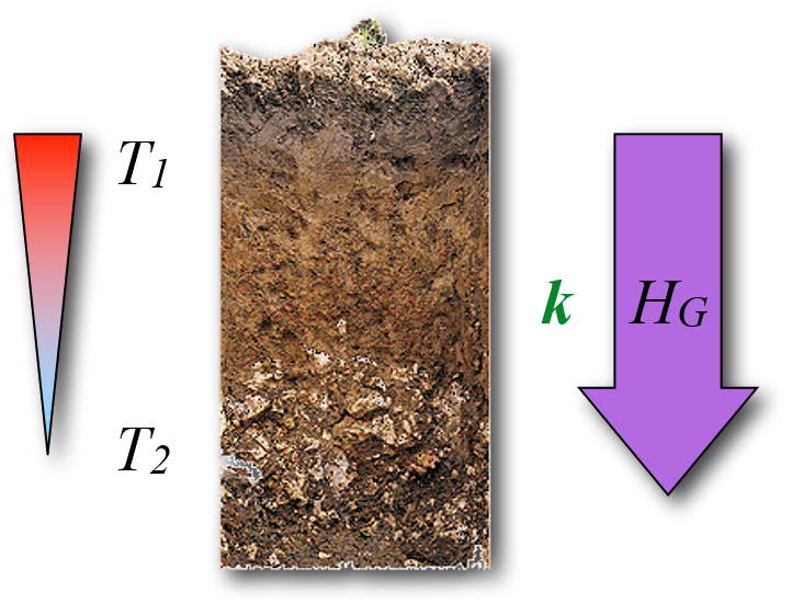
Fourier’s Law

Gives us the flux density of conducted heat (e.g., soil heat flux \(H_g\)) as a function of the temperature gradient and the thermal conductivity (\(k\)) in W m^-1 K^-1

\[ H_G = -k \small\frac{T_2 - T_1}{z_2 - z_1} \qquad(7)\]

Fourier’s Law

What is the difference between Equation 7 and Equation 5?

Thermal Conductivity \(k\)

A metric, given in W m^-1 K^-1, that indicates how well heat conducts through an object. Influenecd by conectivity, homogeneity, and density of the object.

• Mineral matter is a good conductor
• Water is intermediate
• Air is very poor

Table 2: Thermal conductivity of selected substances

Material	k W m-1 K-1
Air	0.025
Water (liquid)	0.590
Ice	2.100
Quartz	8.800
Clay minerals	2.900
Organic matter	0.250
Stainless steel	21.000
Copper	380.000

Unfortunately k is not a simple constant for a given soil. It varies both with depth and with time. However if we restrict ourselves to bulk averages k depends upon the conductivity of the soil particles, the soil porosity, and the soil moisture content. Of these the soil moisture content is the only short-term variable for a given soil.

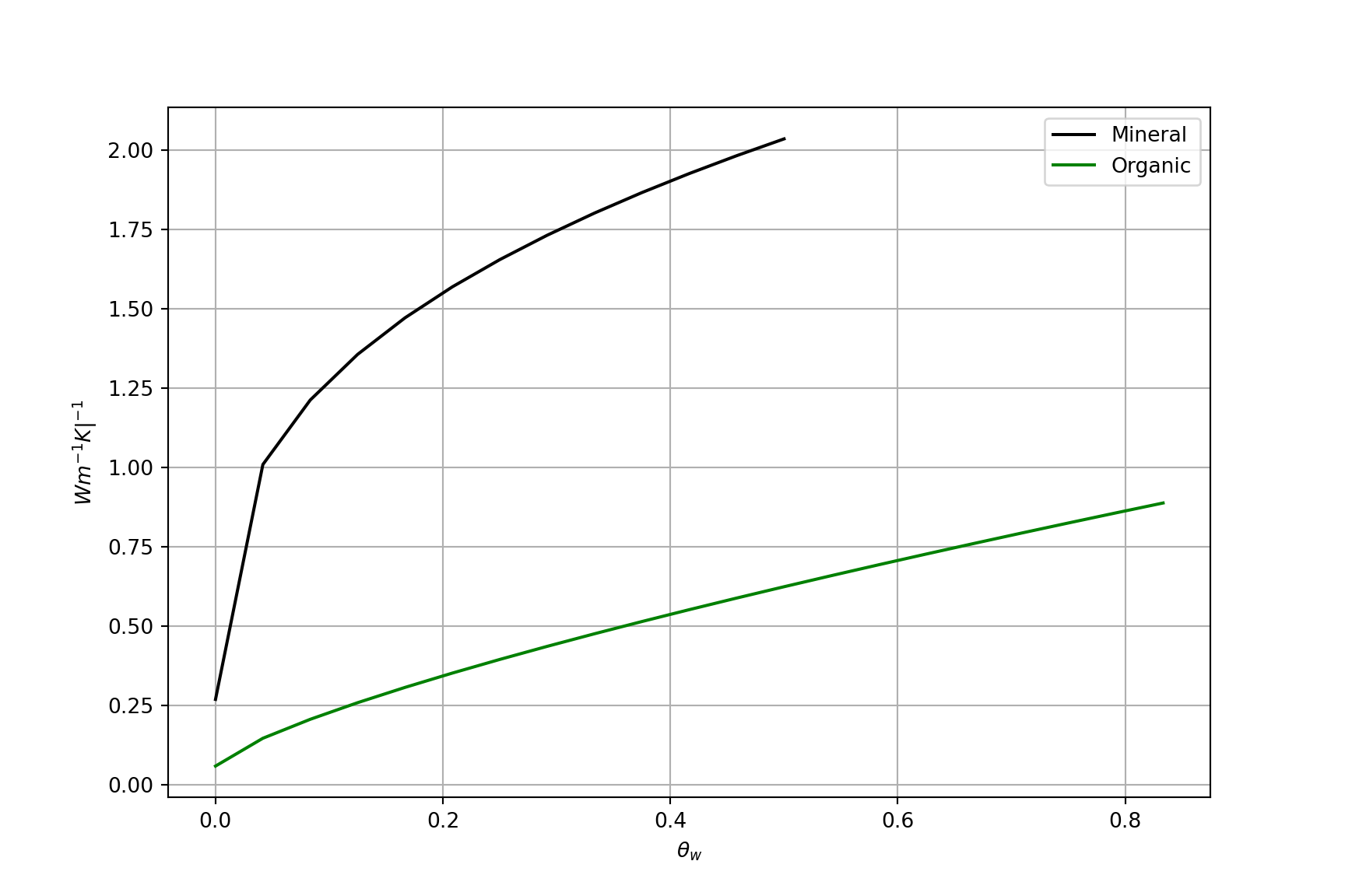
\(k\) vs. \(\theta_w\)

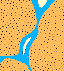
A non-linear relation exists between \(k\) and soil water content (\(\theta_w\))

• Adding water to dry soil (a) initially causes k to increase rapidly – rapid increase in area of contacts between soil particles resulting from water film.
• As more water (b) is added, k increases less rapidly – area of contacts increases more slowly per unit of water added (i.e. diminishing returns).

First, coating the soil particles increases the thermal contact between grains. Second, since the soil pore space is finite the addition of pore water must expel a similar amount of pore air. This means replacing soil air with a substance whose conductivity is more than an order of magnitude greater.

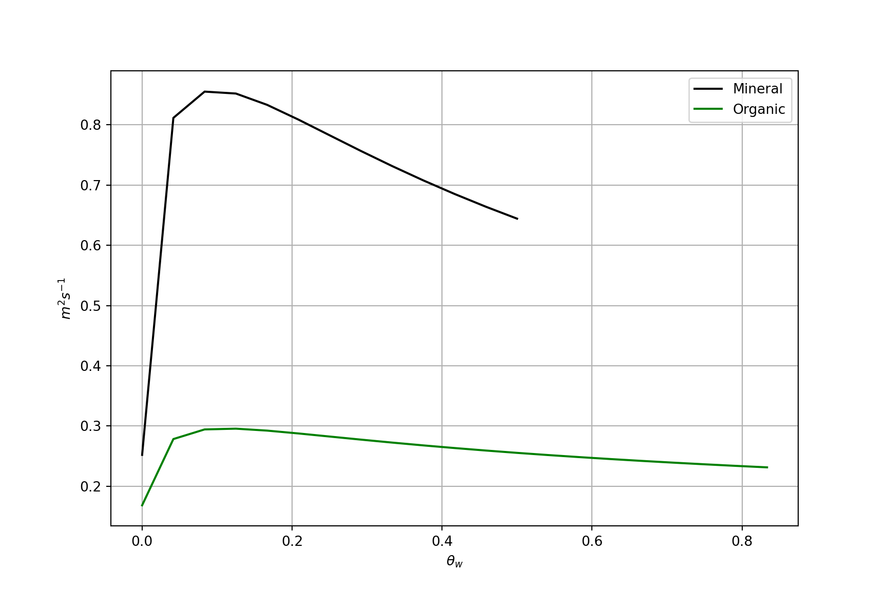
\(k\) vs. \(\theta_w\)

Thermal diffusivity \(k\) of soil vs. volumetric water content \(\theta_w\)

Mineral matter is a good conductor OM has lower thermal conductivity

Thermal diffusivity \(K\)

Thermal diffusivity K – indicates how quickly soil at depth will warm or cool in response to heating or cooling at the surface. It tells us how fast a temperature wave will diffuse or travel downward into a soil.

• It’s units are m² s^-1 and it is defined as:

\[ K = \frac{k}{C} \qquad(8)\]

It controls the speed at which temperature waves move and the depth of thermal influence of the active surface Analogous to the rate of spread of the ripple area after a stone is thrown into a pool. Shows that thermal influences are directly proportional to the ability to conduct heat (k) but inversely proportional to the amount of heat necessary to effect temperature change (C). Thermal diffusivity may be viewed as a measure of the time required for temperature changes to travel.

Why the curious shape?

Thermal diffusivity \(k\) of soil vs. volumetric water content \(\theta_w\)

Peat = much lower thermal conductivity & lower heat capacity; also thermal conductivity had a less pronounced response to increase VWC. Soils with high diffusivities allow rapid penetration of surface temperature changes and permit these effects to involve a thick layer. For the same heat input the temperature regimes of soils with high diffusivity are less extreme than for soils with low diffusivities. By day the surface heating is used to warm a thick layer of soil, and at night the surface cooling can be partially offset by drawing upon heat from a similarly thick stratum. Soils with poor diffusivities concentrate their thermal exchanges only in the upper-most layer, and consequently experience relatively extreme diurnal temperature fluctuations. Therefore, in general a wet clay has a conservative thermal climate, whereas an almost dry peat is extreme.

Measuring Soil Heat Flux

Theoretically, soil heat flux could be simply measured using a vertical array of thermocouples using Fourier’s law.

Measuring Soil Heat Flux

Practically, the problem is the variably \(k\) with water content. Requires continuous measurements of soil volumetric water content \(\theta_w\).

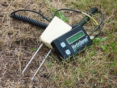
• \(\theta_w\) can be measured precisely in a lab using the gravimetric method or approximated in the field using time domain refractometry (TDR)
  • TDR is an indirect measure based on the travel time of a high frequency electromagnetic pulse through the soil

Measuring Soil Heat Flux

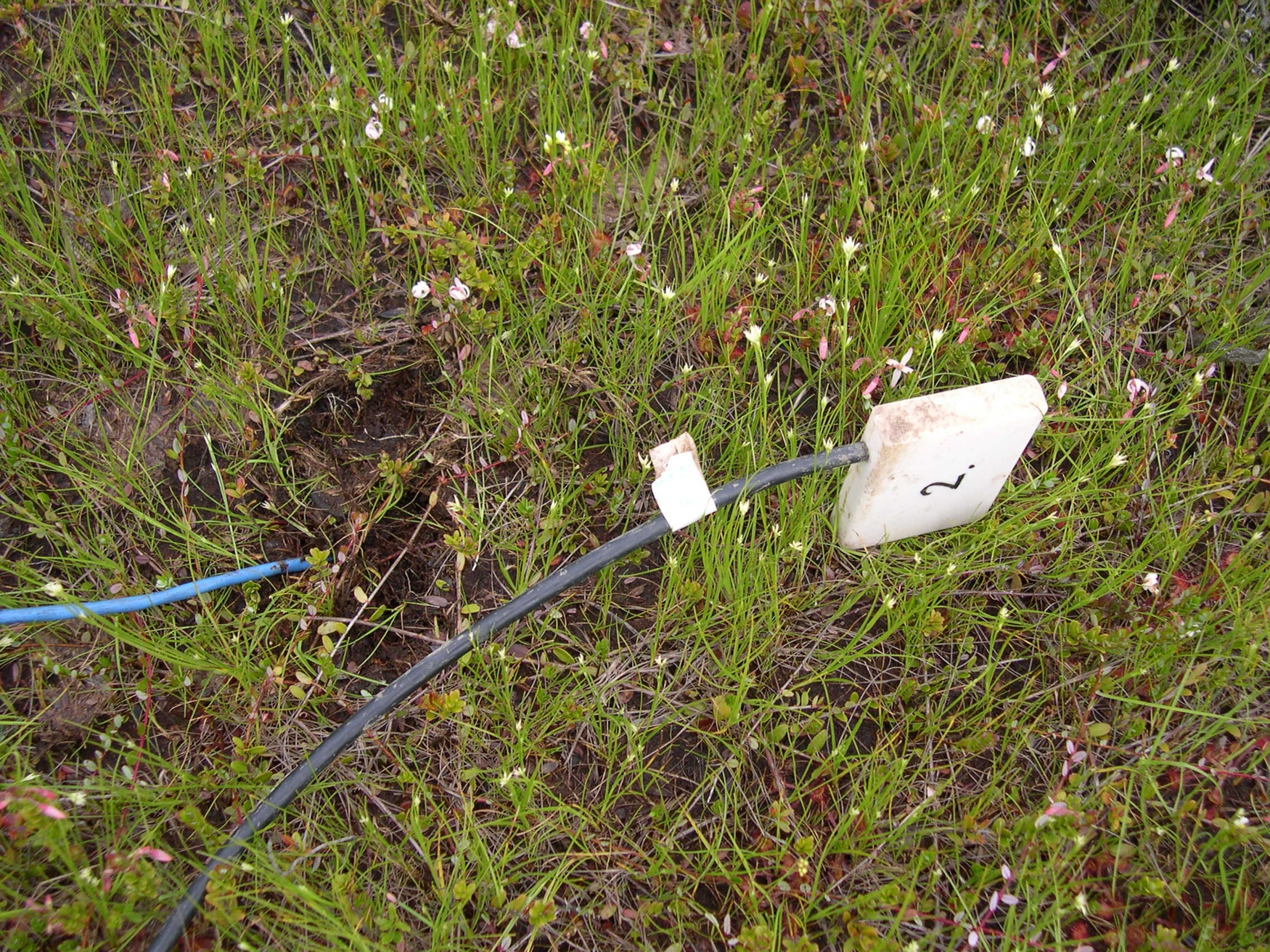
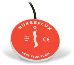
Soil heat flux plates provide a more direct measure of \(H_g\).

Measuring Soil Heat Flux

Soil heat flux plates provide a more direct measure of \(H_g\). The can also be used to estimate the heat capacity \(C\) and thermal conductivity \(k\) of a soil in the field following Equation 5 and Equation 7 respectively.

Estimating \(C\)

\(T_s\) at 5 and 10 cm at 12:00 are 4.18 and 1.98 \(^{\circ}C\) respectively; 1 hour later they are 4.83 and 2.45 \(^{\circ}C\) respectively. Mean \(H_g\) over the interval is 18.035 \(W m^{-2}C\). Approximate \(C\)

T_1 = (4.18+1.98)/2 # Average temperature (deg C) between 5cm and 10cm at 12:00
T_2 = (4.83+2.45)/2 # Average temperature (deg C) between 5cm and 10cm at 13:00
H_g = 18.035 # Average soi heat flux (W m-2) at 7.5 cm over the interval 

Delta_T_delta_t=(T_2-T_1)/3600 # Change in temperature over the 3600 s interval
C_s = H_g/.05/Delta_T_delta_t * 1e-6 # Rearrange and solve, and convert from J to MJ

sprintf('C = %.2f MJ m-3 K-1',C_s)

[1] "C = 2.32 MJ m-3 K-1"

Estimating \(k\) (iClicker)

At 12:00 \(T_s\) at 5 and 10 cm are 4 and 2 \(^{\circ}C\) respectively and “instantaneous” \(H_g\) is 15 \(W m^{-2}C\). Approximate \(k\)

T_1 = 4 #C
z_1 = 5 #cm
T_2 = 2 #C
z_2 = 10 #cm
H_g = 15 #Wm-2

# Rearrange Fourier's Law
k = -(z_2-z_1)/(T_2-T_1)*H_g

sprintf('k = %.2f W m-1 K-1',k)

[1] "k = 37.50 W m-1 K-1"

What’s the issue here?

• A Looks correct
• B Didn’t convert from K to C
• C Didn’t convert from cm to m

Soil Thermal Admittance \(\mu\)

The ability of the soil surface to accept or release heat following a change in soil heat flux (\(H_G\)). How well it can “soak it up” without changing temperature much. It is given by:

\[ \mu = \sqrt{k C} \qquad(9)\]

• \(\mu\) is the soil thermal admittance; \(k\) is the thermal conductivity and \(C\) is the heat capacity
  • Note the similarities to thermal diffusivity Equation 8
  • Units: J m^-2 K^-1 s^-1/2

Thermal Admittance and Surface Temperature 

For a change in soil heat flux (i.e., \(\Delta H_G\)), the change in surface temperature (\(\Delta T_s\)) is inversely proportional to \(\mu\) 

• For the same energy added:
  • Soil with a low \(\mu\) warms and cools more rapidly
  • Soil with a high \(\mu\) warms and cools more slowly

\[ \Delta T_s = \frac{\Delta H_g}{\mu} \qquad(10)\]

\(\mu\) vs \(\theta_w\)

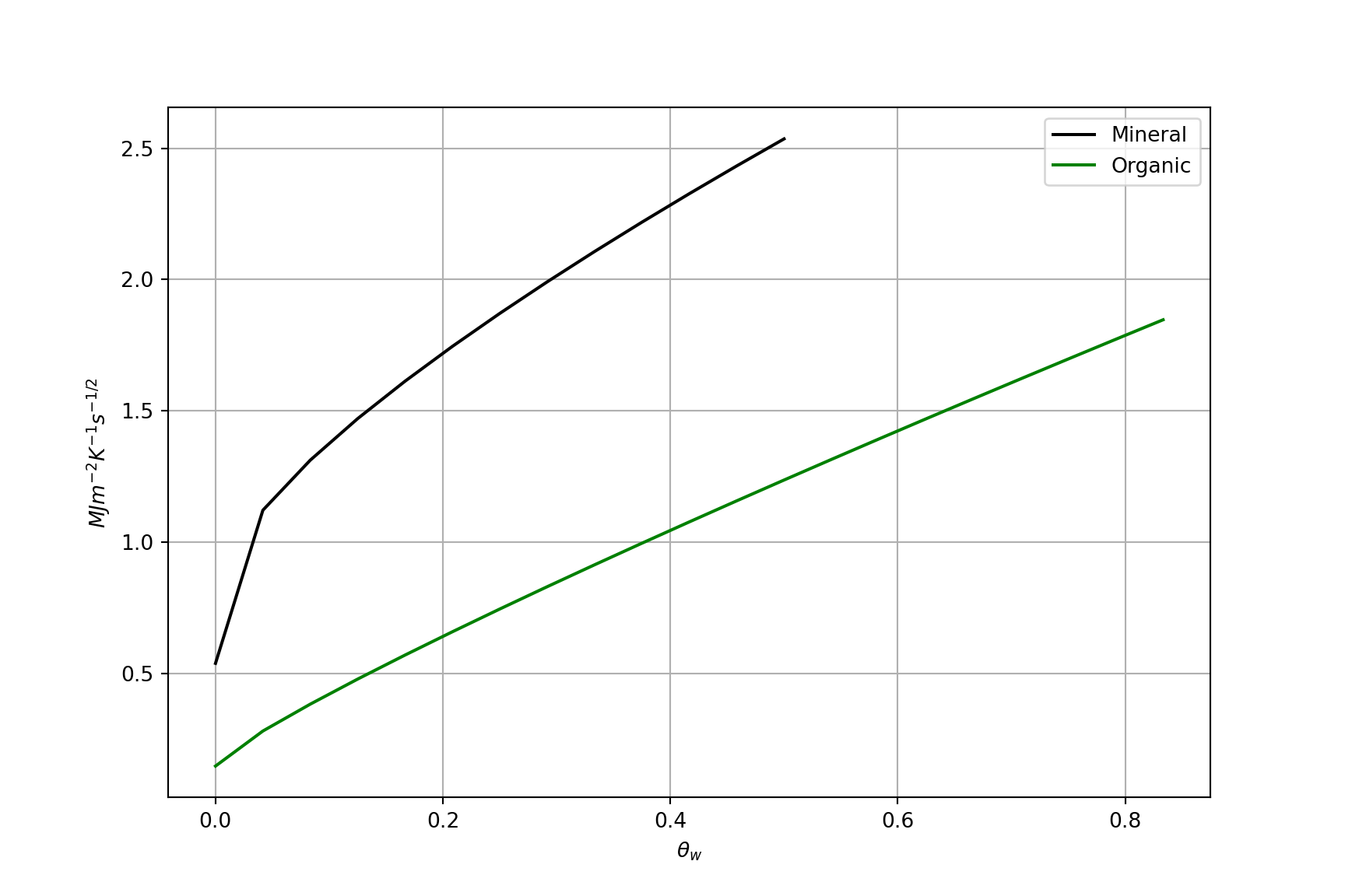
Thermal admittance \(\mu\) of soil vs. volumetric water content \(\theta_w\)

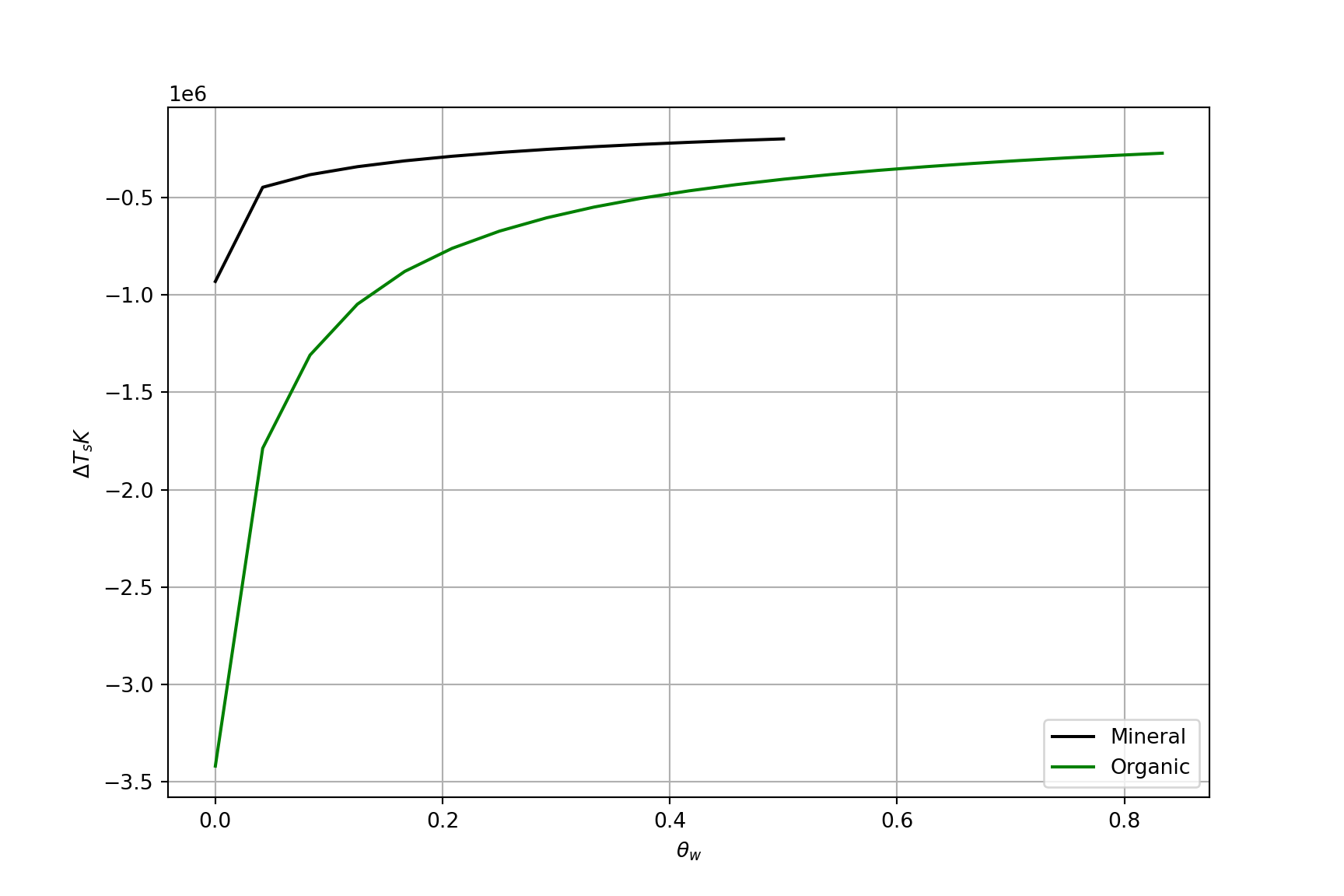
Surface temperature vs \(\theta_w\)

Surface temperature change vs. volumetric water content \(\theta_w\) over a night with 0.5 MJ radiative cooling

Surface temperature vs \(\theta_w\) (iClicker)

Given the plot on the previous slide, at any equivalent value of \(\theta_w\), which soil would better prevent frost damage on a calm clear night?

• A Organic
• B Mineral

Temperature Waves

The variation of temperature with depth can be thought of as waves moving down through the soil in response to radiation “forcing” at the surface.

• There are annual waves, diurnal waves, and waves with shorter periods due to clouds
• In typical mineral soils:
  • Annual waves penetrate to ~ 10 m
  • Diurnal waves to ~ 50 cm
  • Cloud waves to ~ 5 cm

Annual Waves

Mean soil temperatures by month in Burns Bog

Shorter Timescale Waves

Soil temperatures in Burns Bog, June 2023

Summarzign Thermal Properties

How rapidly does a volume warm when a certain amount of energy is supplied?

• Heat Capacity \(C\)

How well does heat conduct from one depth to another for a given temperature gradient?

• Thermal conductivity \(k\)

How rapidly does a soil warm at depth if energy is available at the surface?

• Thermal diffusivity \(K\)

-Heat capacity (C) -Thermal conductivity (k) -Thermal diffusivity (kappa): The thermal diffusivity of the soil is its ability to diffuse thermal influences

Take home points

• Soils are important for storage of heat and water in the climate system.
• Two basic thermal properties regulate the exchange - Heat capacity Cs and thermal conductivity k. From those we can derive thermal diffusivity κ = k / Cs.
• The water content of the soil is significantly altering both C (linearly) and k (non-linearly).